A state-space model for ecological count data
Statistical analyses of ecological multinomial time series to identify environmental drivers and biotic interactions
This work is published in Methods in Ecology and Evolution: Statistical analyses of ecological multinomial time series to identify environmental drivers and biotic interactions (Asena et al., 2026). The model was developed during my postdoc at UW–Madison with Tony Ives and Jack Williams, and is available as the multinomialTS R package.
A blog post accompanying the publication walks through the idea less formally, and I gave an invited talk on it for Methods in Ecology and Evolution. You can watch the talk, and the workshop materials are all open.
Below is an earlier post from when we were developing the model, kept here for context:
Post from 2024-12-01
Over the last couple of years, Tony Ives, Jack Williams and I have been developing a model for estimating coefficients of driver-species relationships, and taxa-taxa interactions from multinomially distributed data. The model works with any data that are multinomially distributed; however, our objective is to be able to understand the drivers of ecological change using palaeo-data.
The point of this work is to go beyond describing patterns of past changes, and get at why ecosystems change. If we can better understand the drivers of change in ecosystems, we can use this knowledge to understand how ecosystems will change into the future under human pressures and environmental change.
A crash course in palaeo-data
There are many forms of data that describe historical changes in environments and ecosystems (e.g., isotopes from ice cores, or diatoms from lake sediments). To reconstruct changes in vegetation, lake sediment cores are often used, and fossilised pollen is extracted from the sediment core. Consider a lake as a big instrument for recording the surrounding environment. Every year, the air is full of pollen from all the wind-pollinated species around the lake. Some of this pollen lands on the lake surface and eventually sinks to the bottom of the lake and leaves a layer like a page in a book (borrowing an analogy from my colleague Rose Gregerson in New Zealand). Every year, another page is added to the book. Each page saying something about the surrounding environment, maybe pine forest takes over from oak woodland, or periods of more fire occur. The book tells the story of the ecosystem.
Figure 1 is a visualisation of the pollen data from a sediment core collected at Story Lake in Northern Indiana. The data are from Schlenker et al., 2024.
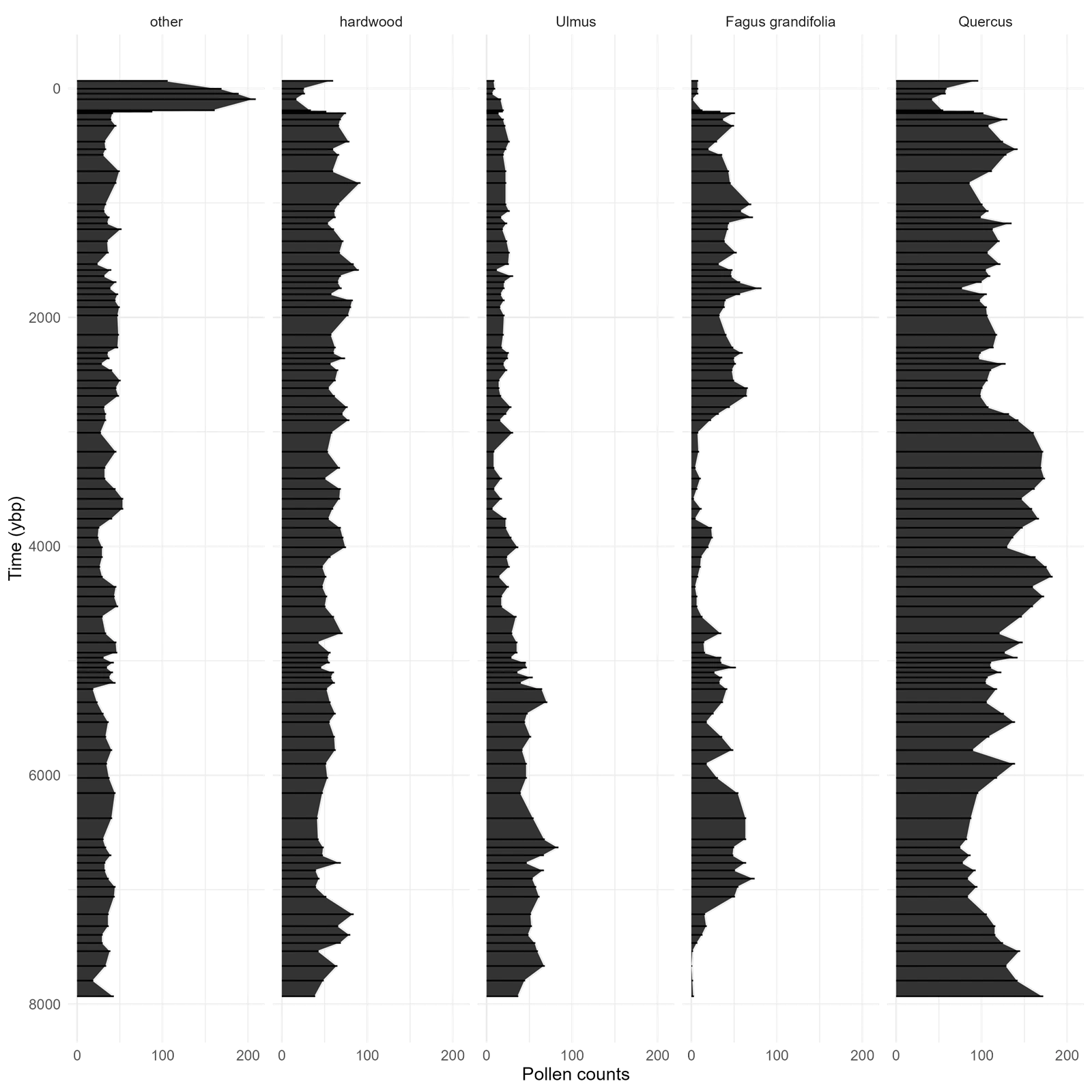
multinomialTS model uses raw counts so I’m showing raw count data. Three key species are plotted (Quercus, Fagus, and Ulmus), along with a group of hardwood species, and a group of all other taxa. The spike in other taxa is caused by an increase in Ambrosia when forests were cleared after Euro-American colonisation of North America.
Our model
These palaeo-data (Figure 1) show patterns of change in the taxa over the time-scale of thousands of years, but we have no direct observations, or experimental evidence of the drivers of change. What this means is we cannot determine, with any certainty, the causes of ecological change over such long time periods. However, it turns out that, with some very fancy maths by Tony Ives, we can generate estimates of the relationships between: (i) environmental drivers (e.g., changes in temperature or moisture) and taxa in the system; and (ii) taxa-taxa interactions. While these estimates cannot be called causal links, they allow us to test (and lend statistical support to) multiple hypotheses about the drivers of ecological change from palaeo-data.
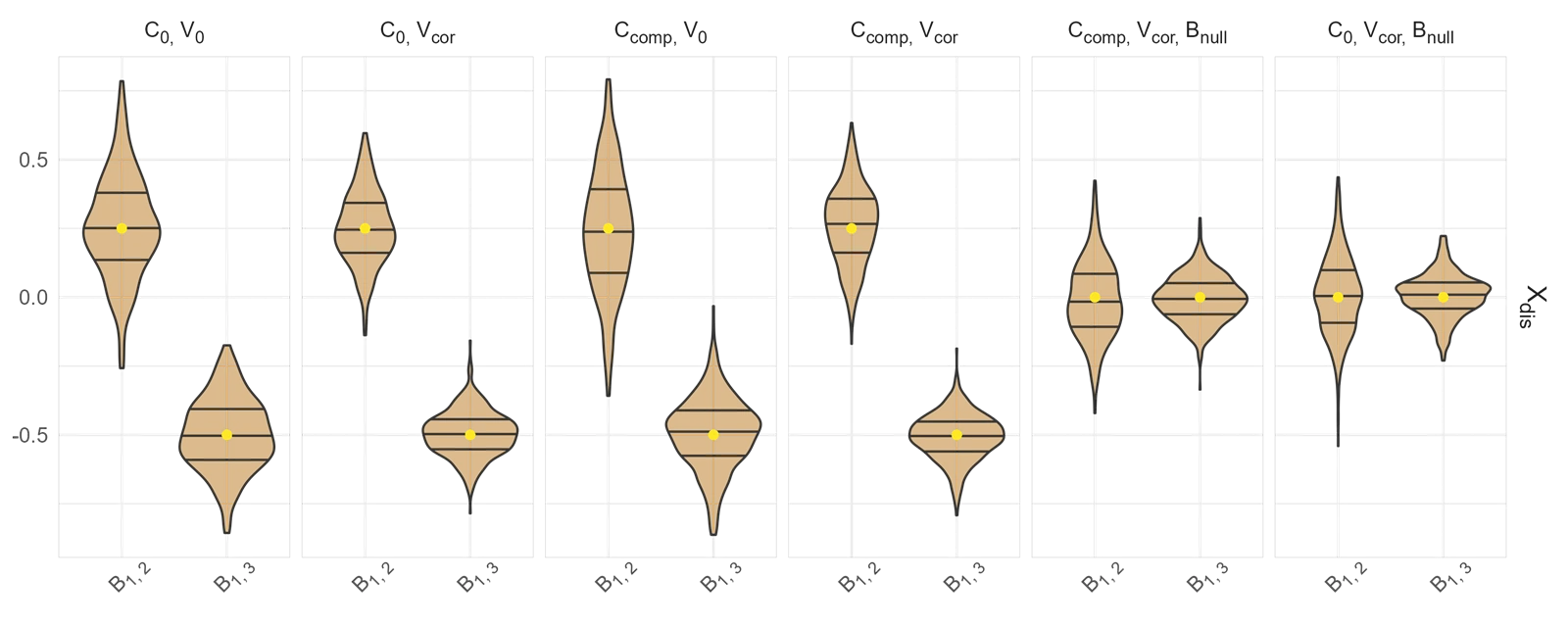
To determine whether the model is recovering accurate estimates of driver-taxa relationships, and taxa-taxa interactions, we turn to simulation. We simulated data with different parameters and assess how well the model recovers those parameters. The whole process is described in detail in the paper, and here is an example from the paper on the success of the model at recovering driver-taxa relationships (Figure 2). This figure (Figure 2) will be a bit tricky to interpret out of the context of the full paper, the key points are that: each sub-plot represents different simulated conditions; each violin within the sub-plots is a simulated taxon; and the yellow dot is the target value that we want the model to estimate. Across many replicate simulations the median recovered value from the model is very close to the yellow dot, this is good!
Outro
This is a very brief summary of the work. A great deal more can be said, but I am keeping these posts as short overviews!
The multinomialTS page collects everything about the package in one place: documentation, install instructions, the paper, and the workshops. For the model itself, start with the package documentation.
I have also given talks and run workshops on this model:
- The
multinomialTSworkshop, the maintained hands-on walkthrough - Slide decks from individual events: workshop talk, ESA 2024, application of the model, ESA 2024, model development, ESA 2023