Modelling palaeoecological community data: a state-space approach
Quinn Asena, Anthony Ives, Jack Williams, and Jonathan Johnson
UW-Madison
2023-08-10
Is the past recoverable from the data?
Palaeoecologists are concerned with questions such as:
- what are the drivers of community change?
- what role do species-environment interactions play?
- what role do density dependence and species interactions play?
- how can palaeoecological information inform present and future ecosystem states?
Palaeoecological proxy data
Proxy data typically:
- comprise mulitple time-series (response):
- e.g., pollen, diatoms…
- include environmental covariates (predictors):
- e.g., isotopic data, charcoal data, lake level…
Pose many statistical challenges:
- Uneven sampling through time
- Time averaging
- Measurement uncertainty
- Relative abundances
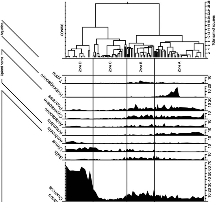
Descriptive approaches
Many descriptive approaches exist for analysing multivariate time-series:
- Cluster analyses: CONISS
- Ordination: PCA, NMDS…
- Machine learning: MVRT, LDA (fancy cluster analyses)
Descriptive methods allow us to see patterns in the data but not determine potential causes of those patterns.
Beyond pattern recognition
The cutting edge in palaeoecology is to establish potential causes of observed patterns in species relative abundances. For example, are observed patterns driven by:
- species interactions?
- climate variability?
- fire regime?
- …
This is what we want to know if we are to use palaeoecology to inform management of contemporary ecosystems or inform potential future ecosystem states. No easy task!
State-space modelling
State-space modelling goes beyond descriptive approaches and attempts to estimate:
- autoregressive / density dependent processes
- interspecific interactions (\(C\) matrix)
- species-environment interactions (\(B\) vector)
- combinations of the above
State-space modelling
State-space modelling attempts to predict the “true” unobservable state of a system from observable variables. It does so via two equations, one that models the process of the system:
Process equation:
\[
Z = B0 + C(Z_{t-1} - B0 - BX_{t-1}) + BX_t
\]
and one that models the observations from the system:
Observation equation:
\[
Y_t = Multinomial(Z_t)
\]
State-space modelling
State-space models are not new to ecology and have been used for:
- estimating animal populations
- animal movement
- plant cover data
- and much more
However, state-space models are not well explored in palaeoecology.
State-space modelling
This new variant of a state-space model:
- uses a multinomial distribution: accepts raw count data
- accepts multiple predictor data streams in the same model: e.g., isotopic data, charcoal accumulation rates, fungal spores…
- simultaneously fits multiple coefficients
- models autocorrelation structure
\[
Z = B0 + C(Z_{t-1} - B0 - BX_{t-1}) + BX_t
\]
\[
Y_t = Multinomial(Z_t)
\]
Can be used to assess a range of possible causes of observed patterns in palaeo-data.
Empirical example
Demonstrating a three-taxon model from Sunfish Pond:
unpublished data: not presenting the dataset, focusing on the modelling approach (Johnson et al., unpub)
ACES project interested in abrupt transitions between dominant species
Jonathon Johnson (JJ)
![]()
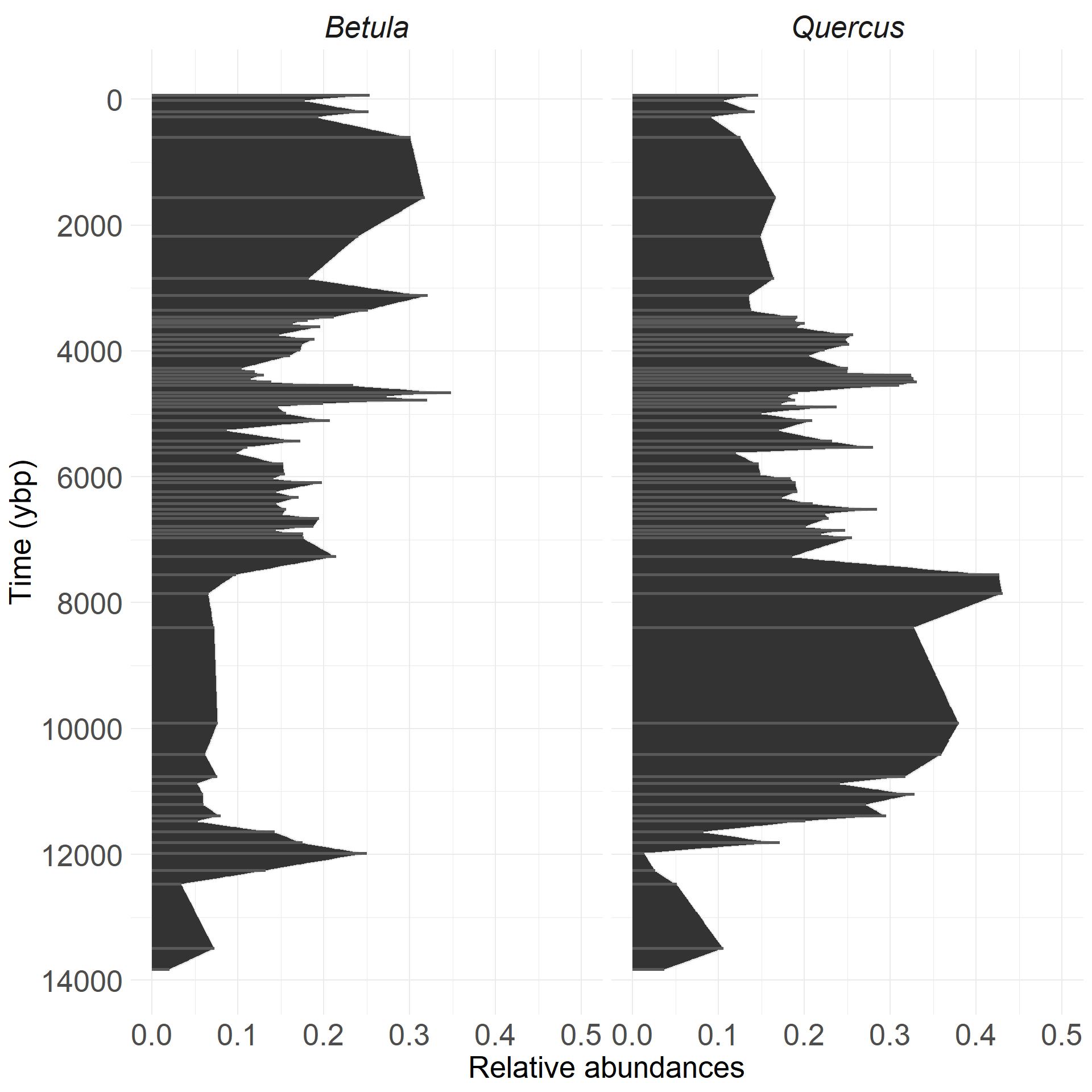
Empirical example
This example is a three-taxon model:
- two focal species (Betula and Quercus)
- third ‘species’ is an aggregate of all other species
- we fit species interactions
- estimate species change through time
Remember, this is a multinomial problem which accounts for unavoidable correlations in frequency data.
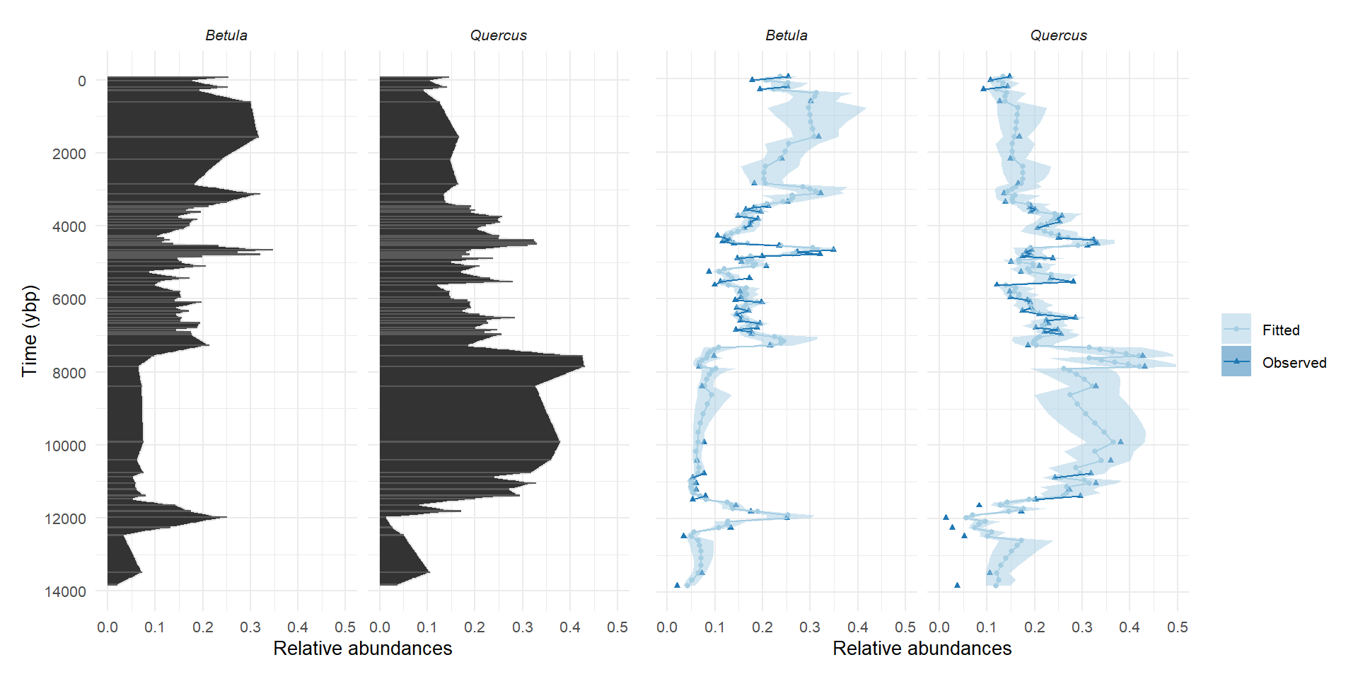
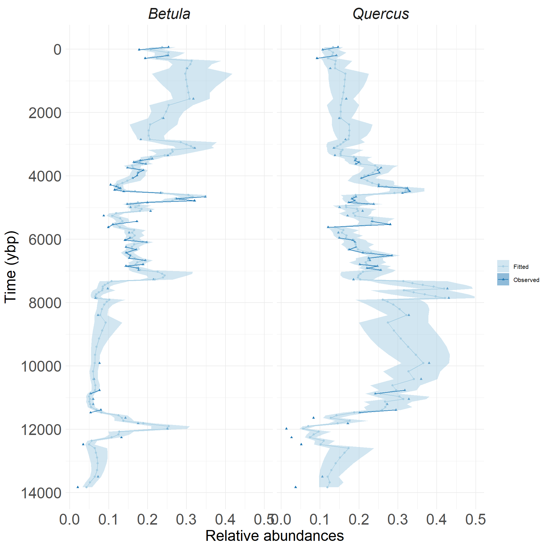
Time-forward model enables uneven intervals
![]()
Johnson et al., unpublished
Species interaction estimates
\(C\) matrix
         other Quercus Betula
other   -0.074   0.000  0.000
Quercus  0.000  -0.006  0.121
Betula   0.000  -0.702 -0.459
columns = abundance; rows = change in abundance
density dependence on the diagonal
Quercus-Betula -0.7 means that abundance of Quercus affects the change in Betula abundance
Estimating the effect of covariates
Estimate of change over time
\(B\) vector
 other Quercus Betula
     0   0.048 -0.532
Overall:
- Quercus increases with time
- Betula decreases with time
- estimates are relative to “other” taxa
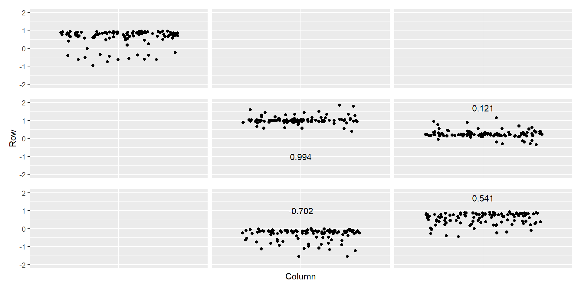
Evaluating the model with simulated data
Evaluating the model with simulated data
\(C\) matrix estimates vs inputs
![]()
Hypothesis testing
We cannot determine with certainty, outside of simulation, causation from palaeo-data.
What we can do is:
- set up multiple working hypothese (Chamberlin, 1897)
- couple descriptive methods with inferrential ones
- assess which results lend support to the likelihood of each hypothesis being true
Given the data at hand the interaction matrix (\(C\)) indicates some competition between Quercus and Betula. Such an inference lends support to one hypothesis.
Acknowledgements
ACES team:
Jack Williams, Tony Ives, Angie Perotti, Nora Schlenker, Sam Wiles, Amanda Toomey Bryan Schuman, David Nelson, Jonathon Johnson
National Science Foundation
UW-Madison