State-space modelling
One of the primary goals of this model is to be able to test multiple hypotheses about the data and lend statistical support to the different hypotheses.
This state-space approach allows us to estimate coefficients for taxa interactions and driver-taxa relationships, that we don’t get from methods such as ordination or cluster analysis.
We recommend this method as complimentary to other methods, as both have their advantages.
Work with uneven time-intervals between observations, and multinomially distributed data
Today’s objectives
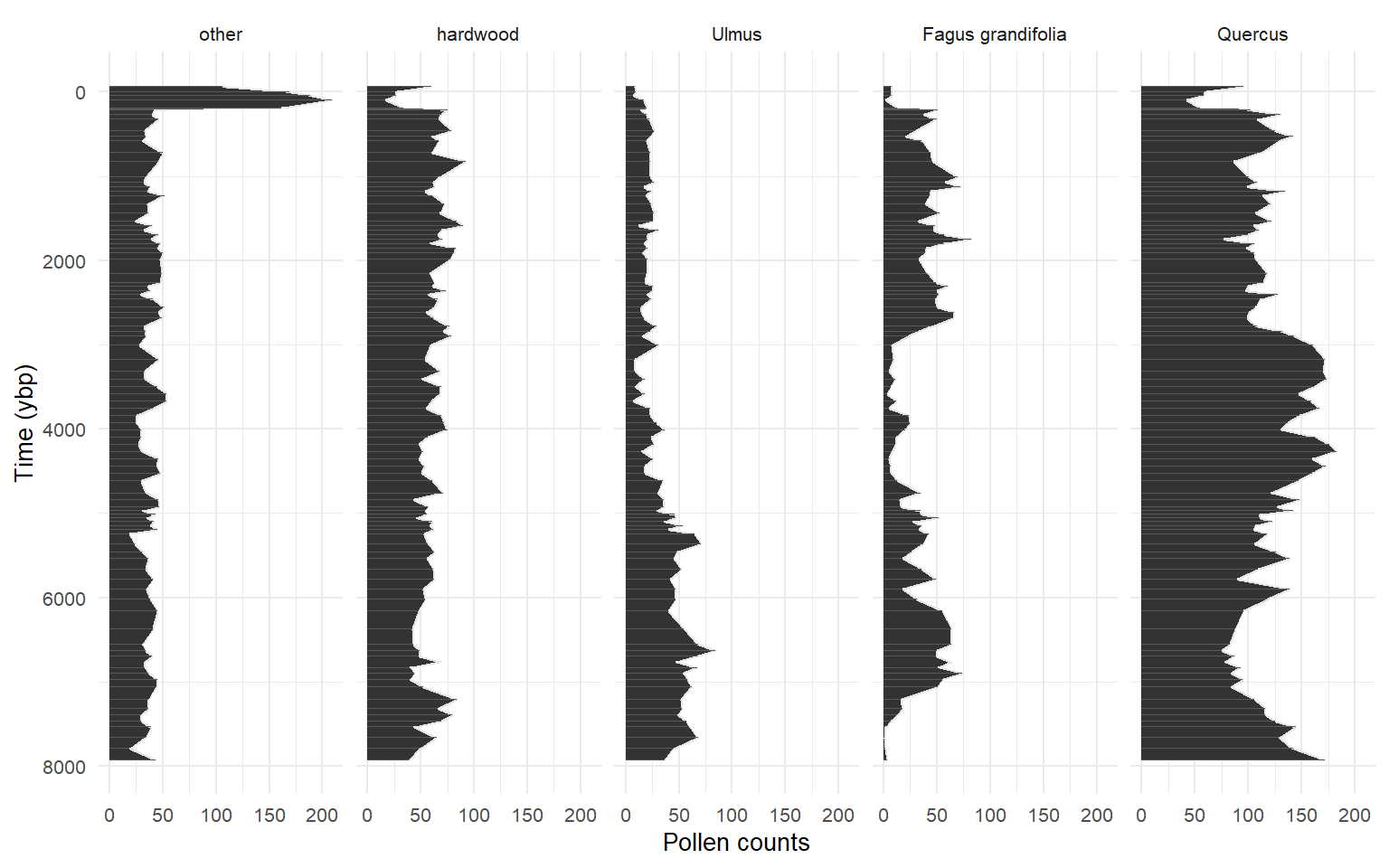
- Learn the data structure for
multinomialTS
- Understand how to fit
multinomialTS
- Finding starting values with
mnGLMM()
- Fitting
mnTS()
- Fit
mnTS() to multiple hypotheses
- Assess resulting models
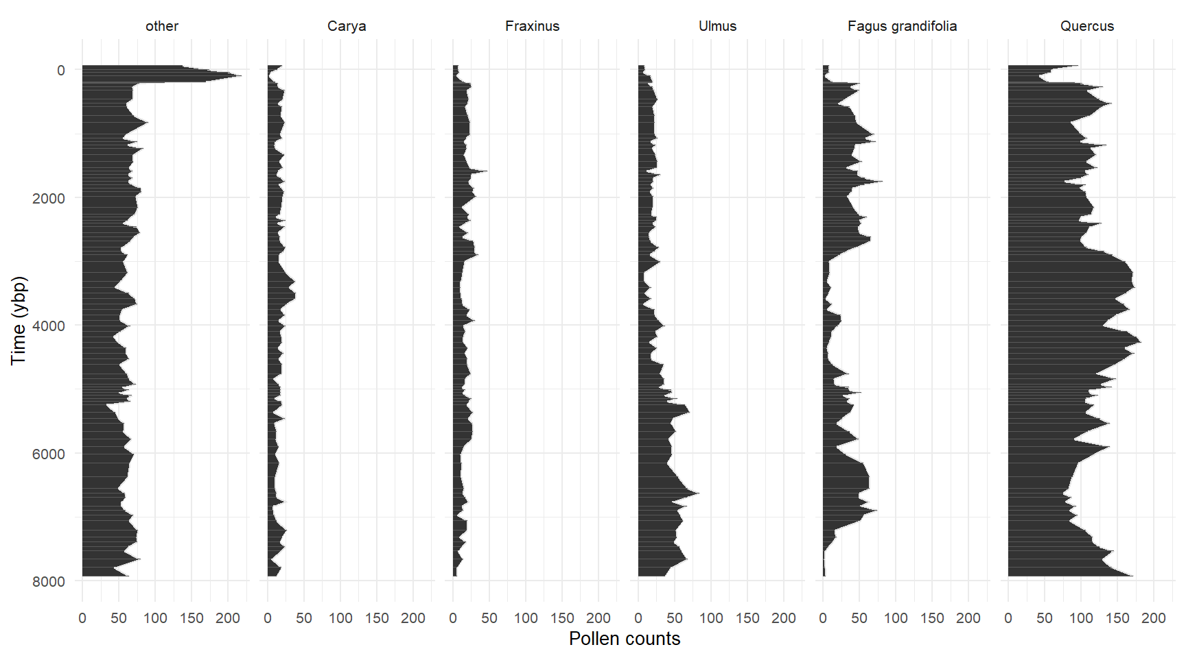
Multinomial and relative abundance data \(Y\)
- Multinomial distribution models the probability of counts for each side of a \(k\)-sided dice rolled \(n\) times
- Individuals counted from each of \(k\) species when \(n\) counts total are made
- Relative abundance data mean we can generate estimates for \(n-1\) taxa
- Everything is estimated against a reference group
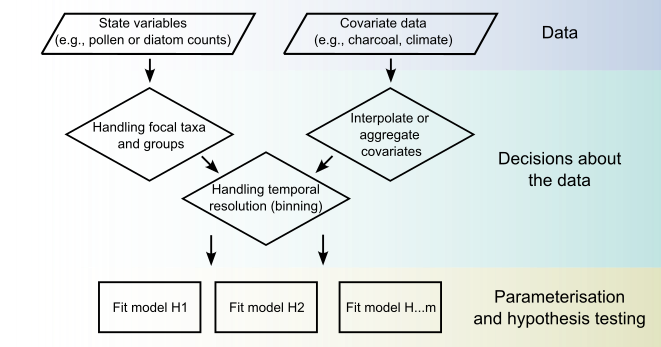
The data
The response variable, \(Y\), is of count-type data. Covariates, \(X\), can be of mixed types (e.g., binary events, or charcoal accumulation rate).
For the model we need two matrices of data:
- \(Y =\) Count data (e.g., pollen, diatoms…)
- \(X =\) Matrix of covariates
Estimated effects
Today, we will look into the estimated parameters \(B\) and \(C\):
- \(B =\) Covariate effect
- \(C =\) Species interactions
Fitting the model to estimate different combinations of parameters allows us to test hypotheses and lend statistical support to them.
For example are species interactions or environmental covariates the primary driver of change?