The modern analogue technique (MAT) is a standard approach for making quantitative inferences about past vegetation and climate from fossil pollen data, and from many other forms of palaeoecological data (Chevalier et al. 2020; Williams and Shuman 2008; Gavin et al. 2003; Overpeck et al. 1985). The MAT relies on reasoning by analogy (Jackson and Williams 2004), in which it is assumed that two compositionally similar pollen assemblages were produced by similar plant communities, growing under similar environments. The similarity of pollen assemblages is determined by the calculation of dissimilarity metrics.
The MAT can also be thought of as a non-parametric statistical technique, called a \(k\)-nearest neighbours algorithm. It is a simple form of machine learning. Each fossil pollen assemblage is matched to 1 or more (\(k\)) modern pollen assemblages, then is assigned the ecological and environmental characteristics associated with those modern analogues.
The MAT is a popular approach for reconstructing past environments and climates, due to its relative simplicity and intuitive appeal. However, like any algorithm, if used unwisely, it can produce spurious results. More generally, when reasoning by analogy, be careful! Analogies are always incomplete and imperfect, and you must use your critical judgement to determine whether these imperfections are minor or serious.
To reconstruct past environments using the MAT, we need three datasets:
Modern species assemblages.
Modern environmental variables.
Fossil species assemblages.
The MAT follows four basic steps:
Calculate dissimilarities between a fossil species assemblage \(i\) and all modern species assemblages in set \(S\).
Discard modern samples with dissimilarities greater than a threshold.
Identify and retain the \(k\) closest modern analogues.
Average the environmental conditions associated with the modern analogues and assign them to fossil sample \(i\).
Note that we are taking a detour into palaeoclimatology for two reasons. First, because palaeoclimatic reconstructions are still a primary use for fossil pollen and other micropalaeontological data. Second, because the MAT and the analogue package, as a dissimilarity-based approach, also lets us explore the novelty of past communities, perhaps of more interest to palaeoecologists than inferred palaeoclimates!
The following section, Section 6.3, takes you through some pretty advanced data wrangling required to match species names between the datasets we will use. However, if you prefer to skip all the wrangling and jump directly to the analyses in Section 6.4, the data have been saved post-wrangling and can be loaded into R directly. Run the ‘Jump point’ code below and portal to Section 6.4.
TipJump point
Load the packages in the next section first, then unfold and run this code to restore the wrangled data and portal to Section 6.4.
Code
# One file holding everything the analysis sections use. It is written at the# end of the data wrangling section, so it cannot go stale relative to it.wrangled <-readRDS("./data/no-analogue-wrangled.rds")mod_pol_harm <- wrangled$mod_pol_harm # modern pollen, harmonised, proportionsdevils_harm <- wrangled$devils_harm # Devil's Lake, harmonised, proportionsdevils_ages <- wrangled$devils_ages # one age per Devil's Lake samplemod_clim_filter <- wrangled$mod_clim_filter # modern climate, aligned row for rowmod_ids <- wrangled$mod_ids # NAMPD sample identifiersmod_sites <- wrangled$mod_sites # NAMPD site names and coordinates
6.2 Getting started
NotePackages required for this section
# Load up the packagesif (!require("pacman")) install.packages("pacman", repos="http://cran.r-project.org")pacman::p_load(dplyr, tidyr, readr, tibble, stringr, neotoma2, analogue)
6.3 Data wrangling
In this case, data are coming from two separate sources, NeotomaDB for the historic pollen data, and the North American Modern Pollen Database (NAMPD; Whitmore et al. (2005)) for both the modern pollen and modern climate variables. These three datasets (Historic pollen, modern pollen, and modern climate data) are required for the MAT. To implement the MAT, the two pollen datasets must contain the same taxa and have identical names for each taxon. Some of the data wrangling required to get two matrices containing the same taxa with identical names for the correct region (as required by the MAT function) is fairly advanced. This type of wrangling is quite common in palaeoecological data-science as you may be dealing with, for example, raw data collected by individuals, or from different databases that are stored in inconsistent formats.
Ready to wrangle? Let’s get the data ready:
TipRespawn code
This is the same Devil’s Lake download used in Chapter 3, so if you have run that chapter the file is already on disk.
# Gated so the API is only contacted when the file is missing. Note the# datasettype filter: site 666 carries five datasets and one of them (3802)# is a modern POLLEN SURFACE SAMPLE rather than part of the core. Downloading# without the filter silently appends a modern sample to the top of a# 14,000 year record.if (!file.exists("./data/devils_dl.rds")) { devils_dl <-get_sites(siteid =666) %>%get_datasets(all_data =TRUE) %>% neotoma2::filter(datasettype =="pollen") %>%get_downloads()saveRDS(devils_dl, "./data/devils_dl.rds")} else { devils_dl <-readRDS("./data/devils_dl.rds")}
The download holds everything Neotoma has for the site. samples() pulls the counts out of it, and does that locally: the API was contacted by get_downloads() above, not here. We keep pollen counted as numbers of grains, from the ecological groups this analysis is about.
devils_samples <-samples(devils_dl) %>% dplyr::filter(ecologicalgroup %in%c("UPHE", "TRSH"), # upland herbs, trees and shrubs elementtype =="pollen", units =="NISP") # counts, not percentagesdplyr::n_distinct(devils_samples$variablename)
[1] 52
Note that in the above code no taxa have been aggregated, and no proportions calculated. Both happen later. The harmonisation table below expects Neotoma’s own names, so lumping Pinus here, as Chapter 5 does for its single-site analysis, would leave the table unable to match any of the three pine taxa Devil’s Lake actually records. And proportions are best calculated after dropping taxa, to avoid re-calculating.
We will use the North American Modern Pollen Database (NAMPD) to create modern analogues (Whitmore et al. 2005). The NAMPD includes both modern surface pollen samples and climate measurements. It is not (yet) accessible through Neotoma, but a copy is saved in the data directory of this book, so we can read it from there. It is always good to keep your own copy of data you depend on: servers are not maintained forever, and datasets are sometimes revised or withdrawn.
The modern datasets include the whole of North America and need to be filtered for the Eastern US so that the taxa are relevant to those in Devil’s Lake. We’re first going to filter by longitude, then select by taxa so that we have a matching matrix of species between Devil’s Lake palaeo-data and the modern surface samples from the NAMPD. We are going to keep all data East of 105°W, see Krause et al. (2019) and Williams et al. (2001) for details.
# Several columns hold information the MAT does not use# Keep the site identifier and the taxon counts only.mod_pol_east <- mod_pol %>%filter(LONDD >=-105) %>%# keep sites east of 105 degrees westselect(ID2, ABIES:XANTHIUM) # ID2 plus the 134 taxon columns# The site names and coordinates are dropped by that select(), so keep a small# lookup table. We need it later to identify particular samples by name.mod_sites <- mod_pol %>%select(ID2, SITENAME, LATDD, LONDD)
We will also filter the modern climate records by the same ID to match the modern pollen records.
Now the tricky part. The two datasets do not use the same taxon names, and they do not identify pollen to the same taxonomic level. We have provided a harmonisation table that accounts for the differences between the two datasets to help with creating the matching historic/modern pollen matrices necessary for the MAT. Creating harmonisation tables that account for naming conventions and taxonomic resolution can be a big job, here are some examples of the challenges of matching databases:
Devil’s Lake records Picea (spruce) to the species-level. The NAMPD splits Picea across three columns, PICEAX (i.e., undifferentiated, genus-level), PICGLAUC (P. glauca) and PICMARIA (P. mariana).
Devil’s Lake records Rhus. The NAMPD has no Rhus column at all, but it does have ANACARDI, the family Rhus belongs to. The two names share no letters, making them hard to find.
Devil’s Lake records Sarcobatus vermiculatus to the species-level. The NAMPD has Sarcobatus to the genus-level.
The NAMPD’s RHAMNACEAE column is not only Rhamnaceae. Its metadata says it combines Rhamnaceae with Vitaceae.
Before the MAT can compare the two pollen datasets, every taxon must have the same naming convention down to the case! Although we have provided a table to crossreference databases, if you need to do this procedure for your own data, several decisions must be made along the way, which do not necessarily have a right answer. Here are some examples of challenges we faced:
What are the dataset’s naming conventions? In the NAMPD a trailing X usually marks an undifferentiated taxon, so PINUSX is “Pinus - Pine undifferentiated”. But the genus names RUMEX and SALIX also end in X and do not indicate undifferentiated taxa. The convention is documented in the workbook’s METADATA sheet, and reading it is more reliable than inferring it from the codes.
Which taxa in which dataset have a finer taxonomic resolution and how do you handle it?Picea the NAMPD has a finer taxonomic resolution than Devil’s Lake, so we summed the pollen counts to match the broader taxonomic resolution of Devil’s Lake. For Sarcobatus Devil’s Lake has a finer taxonomic resolution, so we aggregated Sarcobatus to the genus level at Devil’s Lake to match the NAMPD data.
What happens when no name match exists? In some cases, the family-level was recorded but not the genus- or species- level, for example, Rhus matches to the Anacardiaceae family, Ilex to Aquifoliaceae family, and Morus to Moraceae family. These are particularly tricky to track down!
What do you do with taxa that have no counterpart? Devil’s Lake records Cannabaceae sensu stricto, and the NAMPD has no Cannabaceae column, so those counts are discarded. Angiospermae undiff. (herbs) is unidentified herbaceous pollen with no equivalent, so it goes too. Both are decisions to record rather than problems to solve. It is important to note how impactful removing taxa is to the whole dataset.
An important point to note is that a name-matching algorithm cannot make ecological decisions, and can entirely miss issues like Rhus matching to the Anacardiaceae family. Thus, harmonisation tables, like the one below, require substantial curation!
6.3.2 Matching taxa with the harmonisation table
harmonisation <-read_csv("./data/pollen-harmonisation.csv", show_col_types =FALSE)# One row per harmonised taxon. Each side's original names sit in a single# plus-separated string, so the table stays short enough to read and check.harmonisation %>%select(harmonised_taxon, devils_taxa, nampd_codes, decision) %>%head(10)
# A tibble: 10 × 4
   harmonised_taxon      devils_taxa           nampd_codes              decision
   <chr>                 <chr>                 <chr>                    <chr>
 1 Abies                 Abies                 ABIES                    match
 2 Acer                  Acer                  ACERX+ACNEGUNA+ACPENSYL… sum
 3 Alnus                 Alnus                 ALCRISPA+ALNUSX+ALRUBRA… sum
 4 Amaranthaceae undiff. Amaranthaceae undiff. CHENOAMX                 match
 5 Ambrosia-type         Ambrosia-type         AMBROSIA                 match
 6 Amorpha-type          Amorpha-type          AMORPHA                  match
 7 Apiaceae              Apiaceae              APIACEAE                 match
 8 Artemisia             Artemisia             ARTEMISIA                match
 9 Asteraceae undiff.    Asteraceae undiff.    ASTERCICHO+ASTERX        sum
10 Betula                Betula                BETULA                   match
The decision column records what was done to each taxon: match for a straight one-to-one, sum where several NAMPD columns roll up into one taxon, coarsen where Devil’s Lake was the finer of the two, and drop for the two taxa with no counterpart. Let’s take the harmonisation table and transform it into one row per taxon for each dataset:
harm_nampd <- harmonisation %>%filter(!is.na(nampd_codes)) %>%# Removs taxon that have no matchselect(harmonised_taxon, nampd_codes) %>%# select only necessary columnsseparate_longer_delim(nampd_codes, delim ="+") # split multiple names into individual rowsharm_devils <- harmonisation %>%filter(!is.na(harmonised_taxon)) %>%select(harmonised_taxon, devils_taxa) %>%separate_longer_delim(devils_taxa, delim ="+")# Check the dimensions of both datasetsdim(harm_nampd)
[1] 70 2
dim(harm_devils)
[1] 50 2
Check the output of each table relative to the original harmonisation table:
Now to implement harmonisation itself, which is the same operation on both datasets: pivot to long format, join the table on, then sum the counts within each harmonised taxon. The inner_join is doing quiet but important work here, because any column absent from the table is dropped at that step.
Whenever filtering or joining data it is good to check the dimensions before and after by using dim() to see if the results are what you expect. Some functions like left_join() or full_join() may run without error but produce unexpected results. It is also good to regularly use rowSums() to make sure you are using the correct data type (counts, proportions or percentages), and have not accidentally included age, depth, or ID columns if they should be excluded.
Two housekeeping steps before the analysis. The MAT needs the same taxa in the same order in both matrices, and it needs the climate rows in the same order as the modern pollen rows.
devils_ages <- devils_harm$agemod_ids <- mod_pol_harm$ID2# The climate data must line up row for row with the modern pollen, and the# MAT will not warn you if they do not. In this dataset they already match, but# only because the 94 rows with a missing ID2 also have a missing longitude and# are removed by the eastern filter. Do not rely on that: sort explicitly and# then check.mod_clim_filter <- mod_clim_filter %>%arrange(match(ID2, mod_ids))stopifnot(identical(mod_clim_filter$ID2, mod_ids))# the same taxa, in the same order, on both sidesshared <-sort(intersect(names(mod_pol_harm), names(devils_harm)))mod_pol_harm <-as.matrix(mod_pol_harm[shared])devils_harm <-as.matrix(devils_harm[shared])
6.3.2.1 What the harmonisation cost
Harmonising always loses something, and it is worth reporting how much rather than hoping nobody asks. Both matrices still hold counts at this point, so we can compare them against what we started with.
This is pretty good! We kept almost all of the taxa present in Devil’s Lake, only two of its taxa had no counterpart. The reduction of species in the NAMPD is no surprise given that the data cover the entire eastern U.S. It is also worth seeing which taxa the aggregation changed most, since that is where the harmonisation had the largest effect on the modern data:
Exercise 6.1 The cost table says the NAMPD kept 92.8% of its pollen, so harmonisation discarded 7.2%. That sounds like a lot to lose to a join on taxon names. Find out what it actually was.
The inner_join in harmoniseDatasets dropped every NAMPD column with no row in the harmonisation table, silently and without a message. Those columns are the difference between the two sets of names. The NAMPD also documents what every one of its codes means, and the book ships that sheet, so here are both tools:
# the columns the join threw awayunmapped <-setdiff(names(mod_pol_east)[-1], harm_nampd$nampd_codes)length(unmapped)
[1] 64
# what each NAMPD code actually isnampd_meta <-read_csv("./data/nampd-metadata.csv", skip =41,col_names =FALSE, show_col_types =FALSE) %>%select(code =1, description =3) %>%filter(!is.na(code))
Work out how many grains each of those columns holds and turn that into a percentage of the modern pollen sum. The denominator the cost table used is sum(mod_pol_east[-1], na.rm = TRUE). Sort your answer so the largest losses come first.
Take the eight largest and look each one up in nampd_meta. Search for any whose description you do not recognise, and for each decide whether the plant produces pollen or spores.
The eight are not all the same kind of thing. Add up the share held by the spore and bryophyte producers. How much of the 7.2% do they account for, and how much is left over as a genuine loss of pollen taxa?
Now the judgement. Devil’s Lake was filtered with elementtype == "pollen" and to the ecological groups UPHE and TRSH at the start of this section. Run table(samples(devils_dl)$elementtype) to see what that filter removed, and unique(samples(devils_dl)$variablename[samples(devils_dl)$elementtype == "spore"]) to see how those spores were recorded. Given what you find, is dropping the spore columns from the modern data a loss at all? What would have gone wrong if we had kept them?
6.3.2.2 Converting to proportions
So far, we have been dealing with raw count data but, for the MAT, we need to convert to proportions, and the order matters. Squared chord distance is not scale invariant, so if the rows do sum to one the two datasets are not comparable: a fossil sample whose remaining taxa add up to 0.6 would look artificially far from every modern sample. Dividing before dropping columns is a common and quiet way to get this wrong, but rowSums() provides an easy check!
# Take care that you do not accidentally include an age or depth column# when calculating proportions!mod_pol_harm <- mod_pol_harm /rowSums(mod_pol_harm)devils_harm <- devils_harm /rowSums(devils_harm)# the same data check used in the dissimilarity chapter: both should be exactly 1range(rowSums(mod_pol_harm))
[1] 1 1
range(rowSums(devils_harm))
[1] 1 1
That is the end of the wrangling. Everything the analysis needs is now in RAM, so we save it to disk in one object. We keep all necessary data saved so that all the resources you need exist offline and no API calls are needed to the Neotoma DB (which occasionally undergoes maintenance).
# Written every time this chapter runs, not guarded with file.exists(). These# objects are derived from the code above, so a guard would let the saved file# drift out of step with the chapter while still looking fine.saveRDS(list(mod_pol_harm = mod_pol_harm,devils_harm = devils_harm,devils_ages = devils_ages,mod_clim_filter = mod_clim_filter,mod_ids = mod_ids,mod_sites = mod_sites),"./data/no-analogue-wrangled.rds")
6.4 The Modern Analogue Technique
Now that we have the data we need, and in the format that we need it, we can apply the MAT. If you portaled here and skipped the Data Wrangling in Section 6.3, make sure you load in the pre-formatted data from the jump point in Section 6.1.
6.4.1 Cross-validation
The Modern Analogue Technique needs the same set of taxa in the modern dataset and in the historic pollen data. In Section 6.3.1 we produced: two matrices, mod_pol_harm and devils_harm, with identical columns names (taxa names) and rows that sum to one (relative abundances rather than raw pollen counts). Before reconstructing environmental variables from fossil pollen assemblages, we usually assess how MAT performs in the modern species assemblage. This step is usually referred to as calibration or cross-validation.
In cross-validation, a calibration function is trained on one portion of the modern species assemblages (calibration set) and applied to another portion of the modern species assemblages (validation set). These two datasets are thus mutually exclusive and, possibly, independent. To cross-validate MAT, we usually use a technique called \(k\)-fold cross-validation. In \(k\)-fold cross-validation the modern dataset is split into \(k\) mutually exclusive subsets. For each \(k^{th}\) subset, the calibration dataset comprises all the samples not in \(k\), while the samples in \(k\) comprise the validation dataset. The simplest form of \(k\)-fold cross-validation is the leave-one-out (LOO) technique, in which just a single sample is removed and then all other samples are used to build a prediction for that sample. This procedure is then repeated for all samples. The analogue package uses leave-one-out cross-validation. To assess the model, we can use standard metrics including root mean square error (RMSE) and \(R^2\). Here, we’ll use the cross-validation tools built into the analogue package.
Note that the palaeoSig package, developed by Richard Telford, has additional functions that can test for significance relative to randomly generated variables with the same spatial structure as the environmental variable of interest. We won’t use this package in this chapter, but it’s useful for testing whether apparently strong cross-validation results are merely an artefact of spatial autocorrelation (Telford and Birks 2005).
Now let’s do the analysis! First is the cross-validation of the modern datasets. Using the modern data, we’ll build a calibration dataset and run cross-validation analyses of the calibration dataset. For simplicity, we are going to use January temperatures tjan as our climate variable:
# Select Jan tempsmod_jant <-data.matrix(mod_clim_filter$tjan)# Fit the MAT using only the modern pollen. Named `modpoll_all` because it uses# every modern sample; we are about to find a problem with one of them.modpoll_all <- analogue::mat(mod_pol_harm, mod_jant, method ="SQchord")
print(modpoll_all)
    Modern Analogue Technique

Call:
mat(x = mod_pol_harm, y = mod_jant, method = "SQchord")

Percentiles of the dissimilarities for the training set:

   1%    2%    5%   10%   20%
0.153 0.203 0.299 0.404 0.562

Inferences based on the mean of k-closest analogues:

  k  RMSEP     R2 Avg Bias Max Bias
  1  3.273  0.908   -0.219    2.625
  2  2.933  0.925   -0.262    3.309
  3  2.897  0.927   -0.293    3.332
  4  2.877  0.927   -0.302    3.218
  5  2.869  0.928   -0.317    3.336
  6  2.885  0.927   -0.324    3.597
  7  2.902  0.926   -0.314    3.825
  8  2.961  0.923   -0.321    4.181
  9  3.002  0.921   -0.348    4.291
 10  3.010  0.921   -0.356    4.324

Inferences based on the weighted mean of k-closest analogues:

  k RMSEP   R2 Avg Bias Max Bias
  1   NaN   NA      NaN     2.62
  2   NaN   NA      NaN     3.17
  3   NaN   NA      NaN     3.21
  4   NaN   NA      NaN     3.14
  5   NaN   NA      NaN     3.21
  6   NaN   NA      NaN     3.42
  7   NaN   NA      NaN     3.59
  8   NaN   NA      NaN     3.85
  9   NaN   NA      NaN     3.94
 10   NaN   NA      NaN     3.98
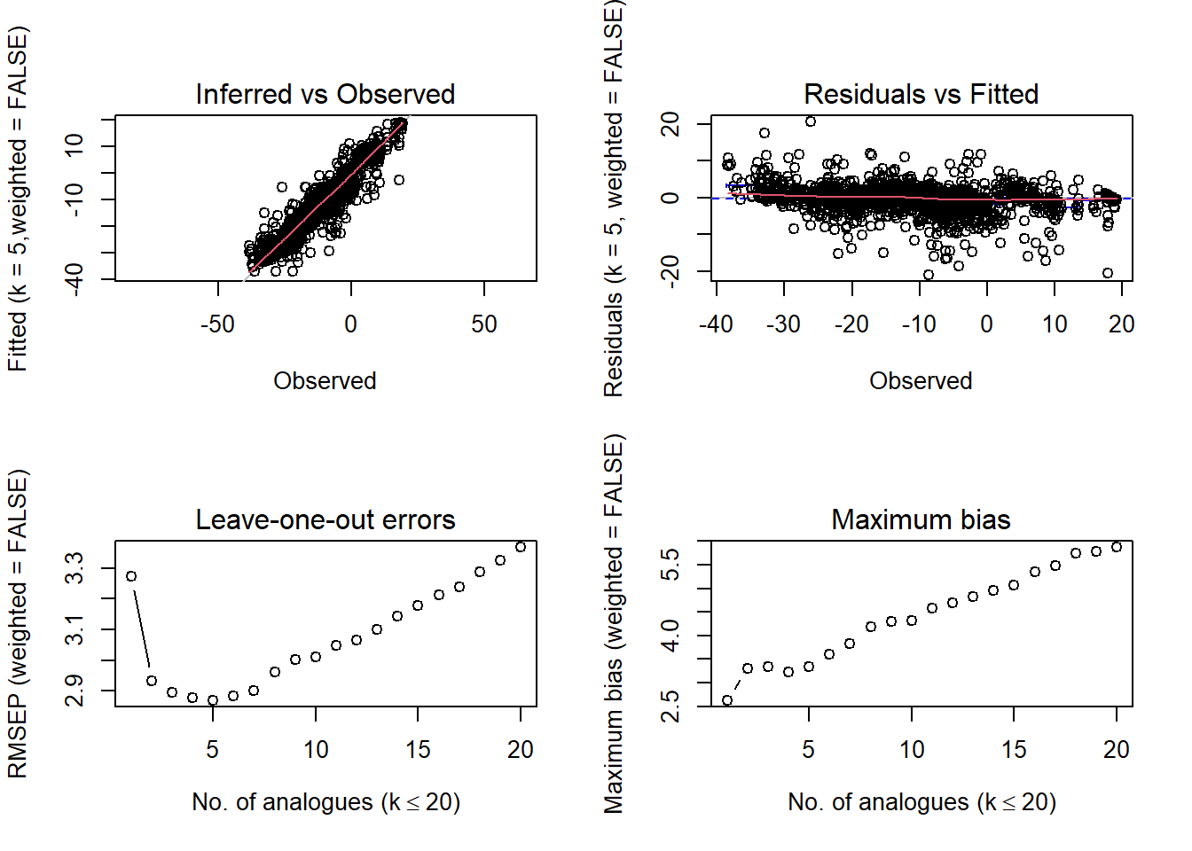
par(mfrow =c(2, 2))plot(modpoll_all)
Figure 6.1: Cross-validation diagnostics for the modern analogue technique applied to mean January temperature, using all 2,594 modern samples. Observed against predicted, the residuals, and the effect of the number of analogues \(k\).
Notice anything off in the summary output?
WarningOh no! 😱
The first table, the plain mean of the \(k\) closest analogues, looks fine. The second table, the weighted mean, is entirely NaN:
Inferences based on the weighted mean of k-closest analogues: k RMSEP R2 Avg Bias Max Bias1NaNNANaN2.882NaNNANaN3.74
No error or warning… This is the most dangerous class of error in the book: no error message, and a plausible-looking answer sitting right next to a broken one. Always read the whole output. The cause is that weighting by inverse dissimilarity requires every dissimilarity to be greater than zero.
Two of the 2,594 modern samples have identical pollen assemblages, so the dissimilarity between them is exactly zero, and one divided by zero is undefined. That single pair poisons the whole weighted-mean column.
So find the duplicate rather than working around it:
# duplicated() works row-wise on a matrix. Round first, because two assemblages# can be identical in every practical sense and still differ in the last bit of# floating-point representation.duplicate_rows <-duplicated(round(mod_pol_harm, 8))sum(duplicate_rows)
[1] 1
# which sites are they? mod_sites holds the names and coordinatestibble(ID2 = mod_ids[duplicate_rows |duplicated(round(mod_pol_harm, 8),fromLast =TRUE)]) %>%left_join(mod_sites, by ="ID2")
Two surface samples about 5.5 km apart, recorded under different site names, with pollen assemblages identical to eight decimal places. Whether that is two genuinely indistinguishable sites or the same sample entered twice by different contributors is a question for whoever curates the database. Either way we cannot use both.
keep <-!duplicated(round(mod_pol_harm, 8))# New objects rather than overwriting the old ones. The full matrices stay# available, which makes the two models comparable and means re-running this# chunk cannot quietly drop a second row.mod_pol_unique <- mod_pol_harm[keep, , drop =FALSE]mod_clim_unique <- mod_clim_filter[keep, ]dim(mod_pol_harm)
[1] 2594 50
dim(mod_pol_unique)
[1] 2593 50
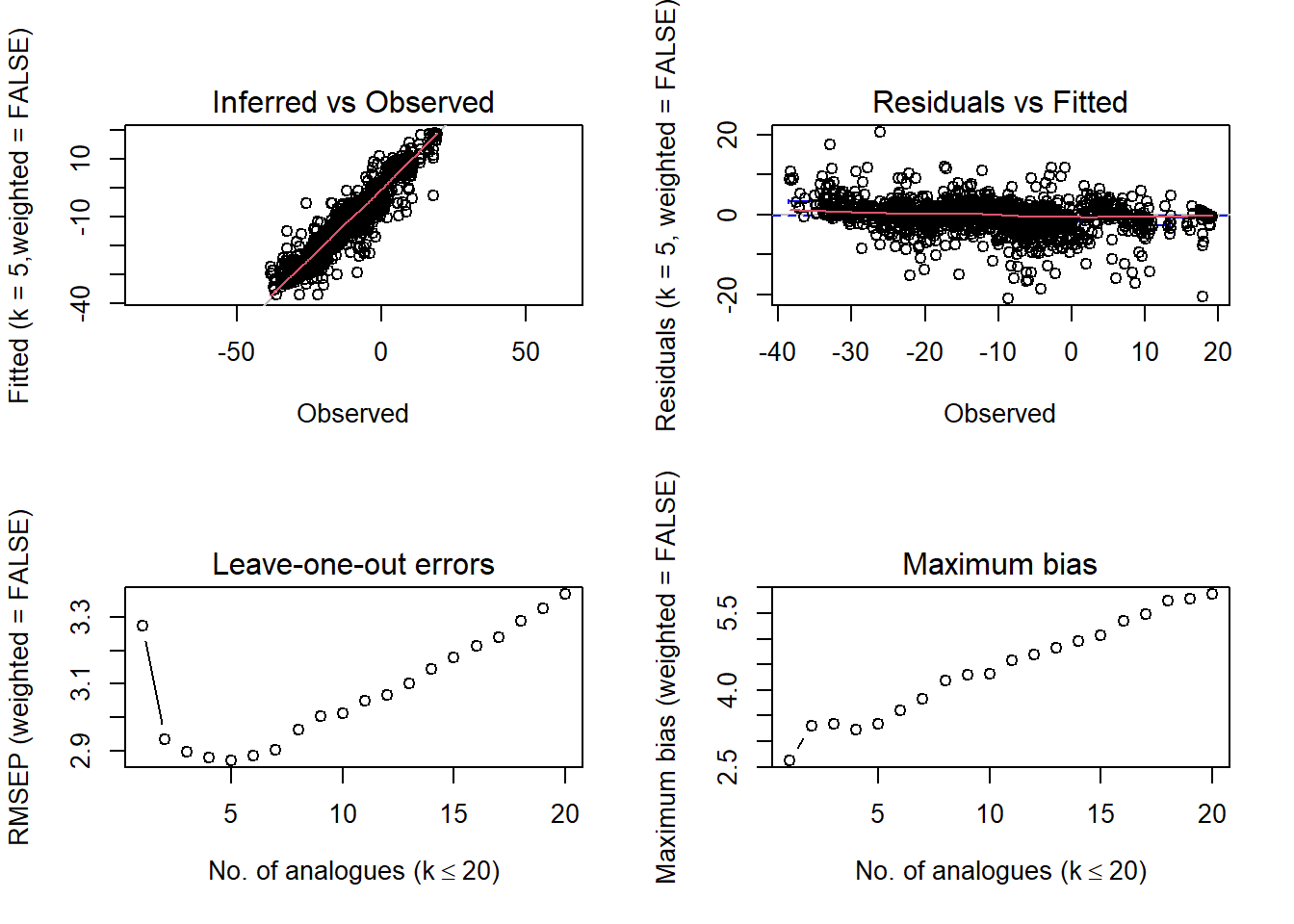
Dropping one sample of 2,594 leaves the mean-based results untouched, so nothing is lost by being careful here: RMSEP at \(k = 1\) moves from 3.379 to 3.380. Now, let’s refit the model and check the output again:
# Select Jan temps for the samples we keptmod_jant_unique <-data.matrix(mod_clim_unique$tjan)# Refit. This is the model the rest of the chapter uses.modpoll_jant <- analogue::mat(mod_pol_unique, mod_jant_unique, method ="SQchord")
print(modpoll_jant)
    Modern Analogue Technique

Call:
mat(x = mod_pol_unique, y = mod_jant_unique, method = "SQchord")

Percentiles of the dissimilarities for the training set:

   1%    2%    5%   10%   20%
0.153 0.203 0.299 0.404 0.562

Inferences based on the mean of k-closest analogues:

  k  RMSEP     R2 Avg Bias Max Bias
  1  3.274  0.908   -0.219    2.625
  2  2.933  0.925   -0.262    3.309
  3  2.897  0.927   -0.293    3.332
  4  2.878  0.927   -0.302    3.218
  5  2.870  0.928   -0.317    3.336
  6  2.885  0.927   -0.324    3.597
  7  2.902  0.926   -0.314    3.825
  8  2.961  0.923   -0.322    4.181
  9  3.003  0.921   -0.348    4.291
 10  3.010  0.921   -0.356    4.324

Inferences based on the weighted mean of k-closest analogues:

  k  RMSEP     R2 Avg Bias Max Bias
  1  3.274  0.908   -0.219    2.625
  2  2.883  0.927   -0.256    3.168
  3  2.814  0.931   -0.279    3.206
  4  2.770  0.933   -0.291    3.138
  5  2.751  0.934   -0.301    3.205
  6  2.751  0.934   -0.306    3.418
  7  2.764  0.933   -0.301    3.595
  8  2.793  0.932   -0.310    3.853
  9  2.827  0.930   -0.330    3.939
 10  2.833  0.930   -0.337    3.975
par(mfrow =c(2, 2))plot(modpoll_jant)
Figure 6.2: The same diagnostics after removing the duplicated modern sample. Compare with Figure 6.1: the mean-based results are unchanged, but the weighted mean is now defined.
Exercise 6.2 The summary for modpoll_jant reports RMSEP, \(R^2\) and bias for every \(k\) from 1 to 10, and the reconstruction later in this chapter is built with k = 10.
Read off the \(k\) that minimises RMSEP, once for the mean and once for the weighted mean. Does the same \(k\) win in both cases?
Rebuild the reconstruction with the \(k\) you chose, using predict(modpoll_jant, devils_harm, k = ...), and plot it against the k = 10 version. How much does the choice actually change the reconstructed temperatures?
RMSEP falls as \(k\) increases and then rises again. Explain both halves of that curve: what goes wrong when too few analogues are averaged, and what goes wrong when too many are?
Exercise 6.3 January temperature is only one of the 69 climate variables in mod_clim_filter. Four others worth trying are tjul (July temperature), pjul (July precipitation), gdd5 (growing degree days above 5°C, a measure of the length and warmth of the growing season) and mipt (an index of soil moisture availability). Note that the column names are lower case.
Refit the MAT for each one, by swapping the variable in data.matrix(mod_clim_filter$tjan) and rerunning analogue::mat(). Record RMSEP and \(R^2\) each time.
Rank the four by predictive skill. Given what you know about which aspects of climate actually control where plants grow, and about how precisely each of these variables can be measured in the first place, is that ranking surprising? Say why.
Much of the information in this chapter comes from Simpson (2007), and we recommend Simpson (2007) for the interpretation of the outputs. The MAT method shares similar considerations as calculating dissimilarity (Chapter 5). With some additional considerations regarding transfer functions:
6.4.2 Novelty and palaeoclimatic reconstruction
Now that we have cross-validated our model on modern samples, we can apply it to the historic pollen assemblage data from Devil’s Lake. The following code calculates and plots the dissimilarity, number of modern analogues, and an inferred temperature reconstruction.
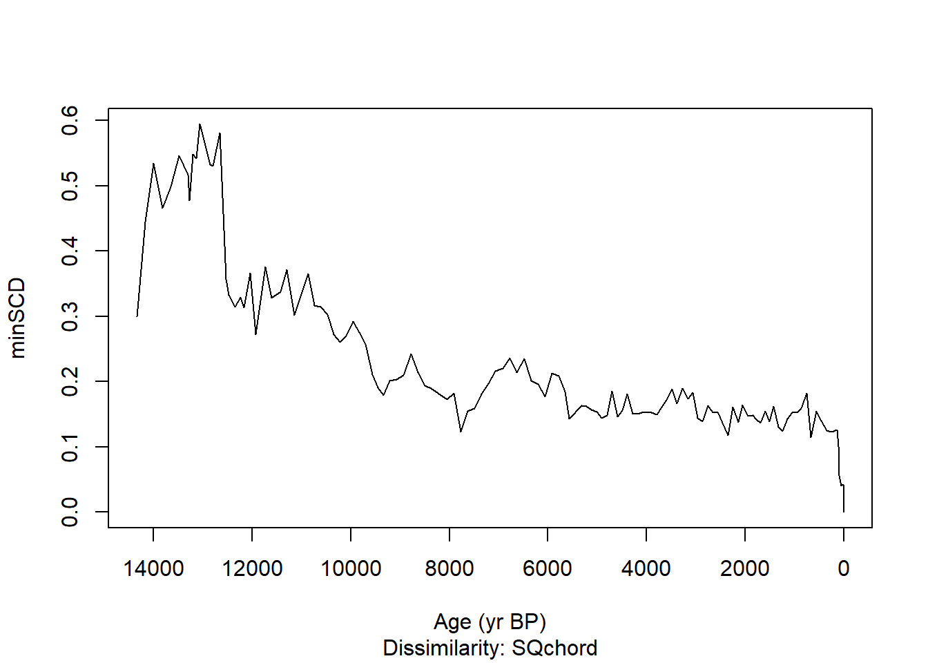
Construct a time series of the minimum SCDs (novelty) for Devil’s Lake.
# Predict temperatures from the fossil data and their modern analogues.# Kept separate from the plot below so that the objects survive even if a# figure chunk is switched off.devil_jant <-predict(modpoll_jant, devils_harm, k =10)devil_mindis <-minDC(devil_jant)
Figure 6.3: Novelty at Devil’s Lake through time, measured as the minimum squared chord distance between each fossil sample and its closest modern analogue. Higher values mean the assemblage is less like anything growing in eastern North America today.
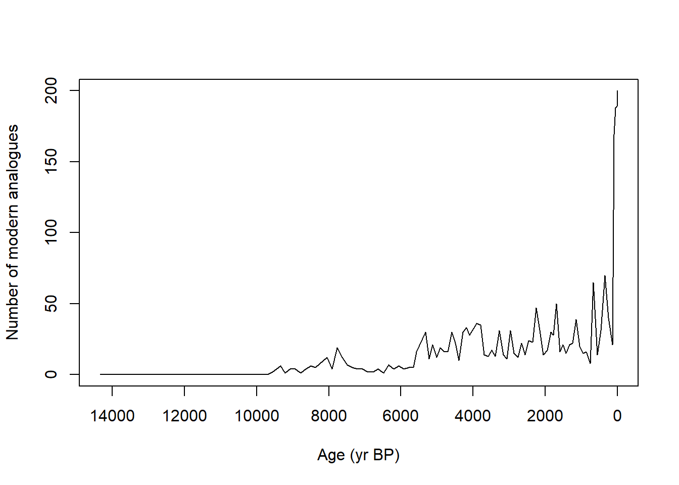
Construct a time series of the number of modern analogues found per fossil sample, using 0.25 as our no-analogue/analogue threshold.
devil_cma <- analogue::cma(devil_jant, cutoff =0.25)# how many fossil samples have no modern analogue at all?sum(devil_cma$n.analogs ==0)
[1] 36
plot(x = devils_ages, y = devil_cma$n.analogs, type ="l",xlim =rev(range(devils_ages)),xlab ="Age (yr BP)", ylab ="Number of modern analogues")
Figure 6.4: The number of modern analogues found for each Devil’s Lake sample, using a squared chord distance of 0.25 as the threshold. Samples with none are the no-analogue assemblages.
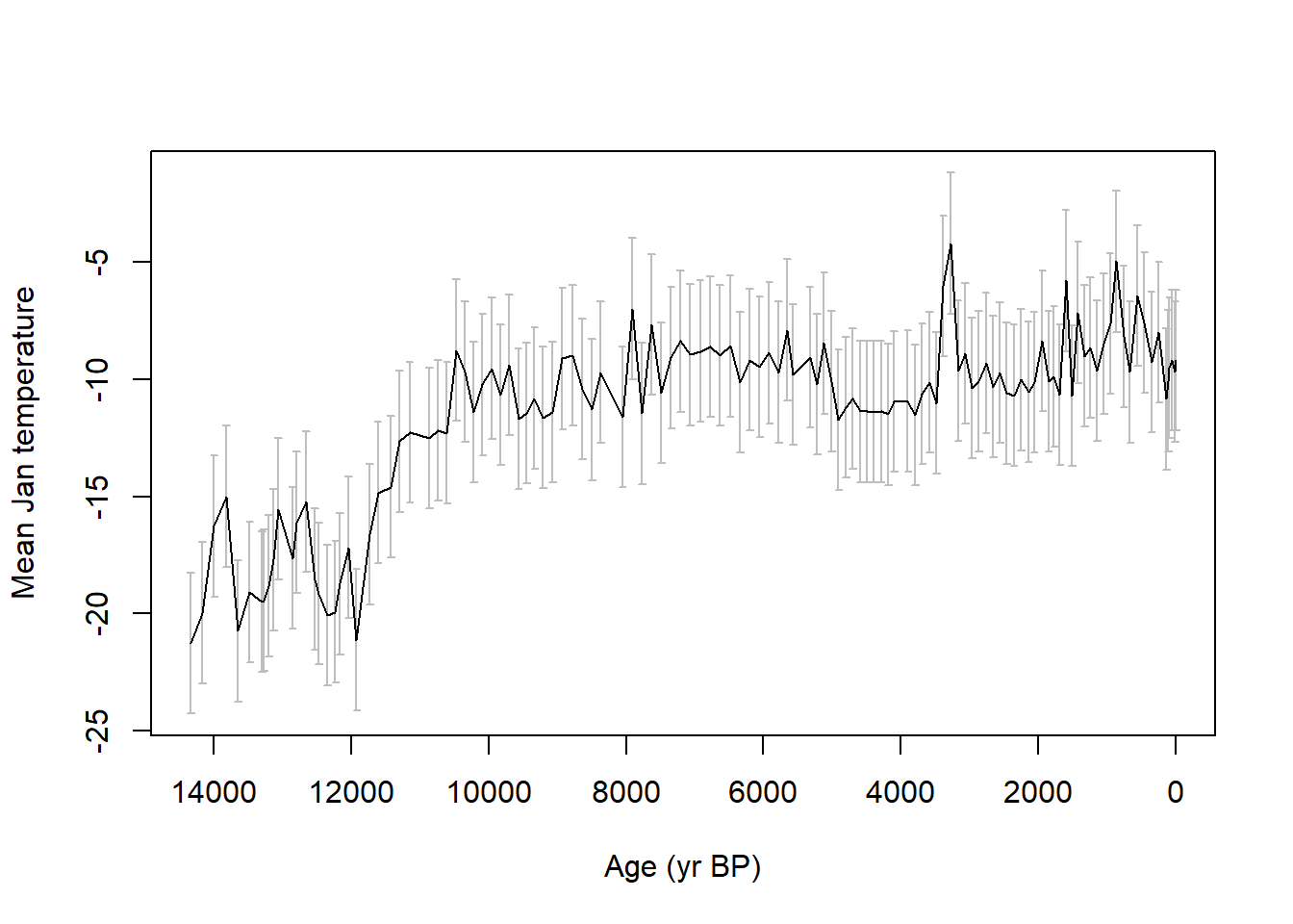
Plot the reconstructed January temperatures at Devil’s Lake:
Figure 6.5: Mean January temperature at Devil’s Lake reconstructed with the modern analogue technique, with error bars. Compare the high-novelty intervals in Figure 6.3 before trusting any part of this curve.
Exercise 6.4 Devil’s Lake is a single record. A reconstruction is far more convincing if a nearby site tells the same story.
Find another pollen site within a few hundred kilometres of Devil’s Lake using the search methods in Chapter 2, and download it with the same gated pattern as the respawn code above. Remember the datasettype filter.
Put it through the harmonisation table and the MAT, then plot its reconstruction against the Devil’s Lake one.
The harmonisation table was built for Devil’s Lake, so its devils_taxa column lists that site’s taxa and no others. Find what your site records that the table has no row for. How much pollen does that cost you, and does it change how much you trust the comparison?
6.4.3 Limitations
Similar to the dissimilarity calculations in Chapter 5:
Chronological uncertainties are not accounted for. See Chapter 3 for how the timing of ecological events may change based on the age-depth model.
Time averaging is not taken into account, and each sample may contain a different time-span of ecological productivity.
Squared chord distance is one of many distance measures available in analogue, and may not always be the most appropriate.
Additionally, transfer functions can themselves be problematic with circular reasoning using vegetation assemblages to infer climate and also inferring how climate affects vegetation! For deeper considerations of reconstructing temperatures using transfer functions see Telford and Birks (2005).
6.5 Conclusion
Remember that a limitation of dissimilarity measures was the lack of covariate data? The MAT includes modern climate combined with modern pollen to predict historic climate. We are now introducing environmental covariates into our analyses!
The exercises take that further, and are worth returning to if you skipped them:
Exercise 6.1, what the harmonisation actually discarded
Exercise 6.3, and which aspects of climate pollen can actually predict
Exercise 6.4, applying the whole workflow to a second record
Chevalier, Manuel, Basil A. S. Davis, Oliver Heiri, et al. 2020. “Pollen-Based Climate Reconstruction Techniques for Late Quaternary Studies.”Earth-Science Reviews 210 (November): 103384. https://doi.org/10.1016/j.earscirev.2020.103384.
Gavin, Daniel G, W.Wyatt Oswald, Eugene R Wahl, and John W Williams. 2003. “A Statistical Approach to Evaluating Distance Metrics and Analog Assignments for Pollen Records.”Quaternary Research 60 (3): 356–67. https://doi.org/10.1016/S0033-5894(03)00088-7.
Jackson, Stephen T., and John W. Williams. 2004. “Modern Analogs in Quaternary Paleoecology: Here Today, Gone Yesterday, Gone Tomorrow?”Annual Review of Earth and Planetary Sciences 32 (1): 495–537. https://doi.org/10.1146/annurev.earth.32.101802.120435.
Krause, Teresa R., James M. Russell, Rui Zhang, John W. Williams, and Stephen T. Jackson. 2019. “Late Quaternary Vegetation, Climate, and Fire History of the Southeast Atlantic Coastal Plain Based on a 30,000-Yr Multi-Proxy Record from White Pond, South Carolina, USA.”Quaternary Research 91 (2): 861–80. https://doi.org/10.1017/qua.2018.95.
Overpeck, J. T., T. Webb, and I. C. Prentice. 1985. “Quantitative Interpretation of Fossil Pollen Spectra: Dissimilarity Coefficients and the Method of Modern Analogs.”Quaternary Research 23 (1): 87–108. https://doi.org/10.1016/0033-5894(85)90074-2.
Simpson, Gavin L. 2007. “Analogue Methods in Palaeoecology: Using the Analogue Package.”Journal of Statistical Software 22 (September): 1–29. https://doi.org/10.18637/jss.v022.i02.
Telford, R. J., and H. J. B. Birks. 2005. “The Secret Assumption of Transfer Functions: Problems with Spatial Autocorrelation in Evaluating Model Performance.”Quaternary Science Reviews 24 (20-21): 2173–79. https://doi.org/10.1016/j.quascirev.2005.05.001.
Whitmore, J., K. Gajewski, M. Sawada, et al. 2005. “Modern Pollen Data from North America and Greenland for Multi-Scale Paleoenvironmental Applications.”Quaternary Science Reviews 24 (16-17): 1828–48. https://doi.org/10.1016/j.quascirev.2005.03.005.
Williams, J. W., and B. Shuman. 2008. “Obtaining Accurate and Precise Environmental Reconstructions from the Modern Analog Technique and North American Surface Pollen Dataset.”Quaternary Science Reviews 27 (7-8): 669–87. https://doi.org/10.1016/j.quascirev.2008.01.004.