# Load up the package
if (!require("pacman")) install.packages("pacman", repos="http://cran.r-project.org")
pacman::p_load(Bchron, splines, ggplot2, dplyr, neotoma2) # splines comes with base R3 Age-depth modelling
3.1 Background
A foundational difference between geology and ecology is that, for geologists, time is an unknown variable that must be estimated with uncertainty. In contrast, most ecologists can assume that the temporal coordinates of their observations are known precisely, with zero uncertainty. Fortunately, geochronologists have a wide variety of natural clocks, thanks to the constant decay rates of radioactive isotopes. Each isotope has a unique decay rate, and so each is appropriate for particular timescales.
For the last 50,000 years, radiocarbon (14C), with its half-life of 5,730 years, is by far the most common form of radiometric dating. (Beyond 10 half-lives, so much of a radioactive substance has decayed away that it becomes immeasurable.) Radiocarbon is the mainstay of Quaternary dating and archaeology.
In Quaternary palaeoecology, radiocarbon dating is expensive: a single sample typically costs $300 to $500, so usually a given lake-sediment record will have only a scattering (ca. 5 to 30) of radiocarbon dates and other age controls. Other kinds of age controls include volcanic ash layers (tephras), 210Pb (half-life: 22.3 yrs), optically stimulated luminescence (OSL) dates, historic events such as the rise in Ambrosia pollen abundances associated with EuroAmerican land clearance, etc. An age-depth model must be constructed to estimate the age of sediments not directly associated with an age control. In multi-site data syntheses, the number of age controls, their precision, and their likely accuracy are all fundamental indicators of data quality (e.g., Blois et al. 2011; Mottl et al. 2021).
To estimate ages for depths lacking a radiocarbon date, an age-depth model is required. Age-depth models are fitted to the available age controls (age estimates with uncertainty for individual depths) and provide estimates of age as a function of depth, for all depths and ages within the temporal bounds of the model.
3.1.1 Getting started
Here we will gain practice in working with age-depth models of various kinds, and assessing their age estimates and uncertainty. We’ll begin with a bit of practice in calibrating radiocarbon years to calendar years and comparing the resulting age estimates from different calibration curves.
NotePackages required for this section
We will be using Bchron for calibration and Bayesian age-depth modelling. Notably rbacon is another commonly used package, see Trachsel and Telford (2017) for a discussion of age-depth models. Remember that you must have packages both installed and loaded; loading a package is usually done via the library(packagename) function. The following code using the pacman package takes care of installation and loading in one go.
3.2 Calibration of radiocarbon dates
A complication in radiocarbon dating is that the initial calculation of a radiocarbon age assumes, by convention, that the amount of radiocarbon in the atmosphere is constant over time (see Bronk Ramsey (2008) for a good overview of how 14C dating works). This assumption is untrue, so all radiocarbon age estimates must be post-hoc calibrated using a calibration curve that is based on compiling radiocarbon dates of materials that have precise independent age estimates (e.g., tree rings, corals). Different calibration curves need to be used for the Northern vs. Southern Hemisphere and for the atmosphere vs. oceans, due to different residence times of 14C in these different reservoirs. For example, atmospheric radiocarbon that diffuses into the surface oceans usually will reside for centuries before phytoplankton biologically fix it through photosynthesis, which will lead marine 14C to be depleted (and ‘too old’) relative to atmospheric 14C. Use the wrong calibration curve and your age estimate will be inaccurate! The IntCal series (IntCal04, IntCal09, IntCal13, IntCal20) is the community standard for calibrating radiocarbon dates to calendar years in the northern hemisphere (e.g., Reimer et al. 2020). The SHCal series does the same job for the southern hemisphere (Hogg et al. 2020). Choosing between them is not optional: use the wrong curve and every age will be biased. The conversion from radiocarbon to calendar years usually further increases the uncertainty of age estimates.
We will start by calibrating a single date together with the curve it was calibrated against. In the figure below, the shaded distribution on the y-axis is the radiocarbon age (i.e., the estimate returned by the lab); the shaded distribution on the x-axis is the probability of a given calendar age; and the diagonal wiggly line is the calibration curve itself. Take a minute to get comfortable with interpreting this figure. The important concept to grasp is how the 14C distribution on the y-axis intersects with the calibration curve to produce the calibrated distribution on the x-axis. You can use the grid lines to visualise the intersection. See how high probability calendar age regions intersect with the peak of the 14C age distribution?
BchronCalibrate(ages = 11553,
                ageSds = 50,
                calCurves = "intcal20") %>%
  plot(includeCal = TRUE)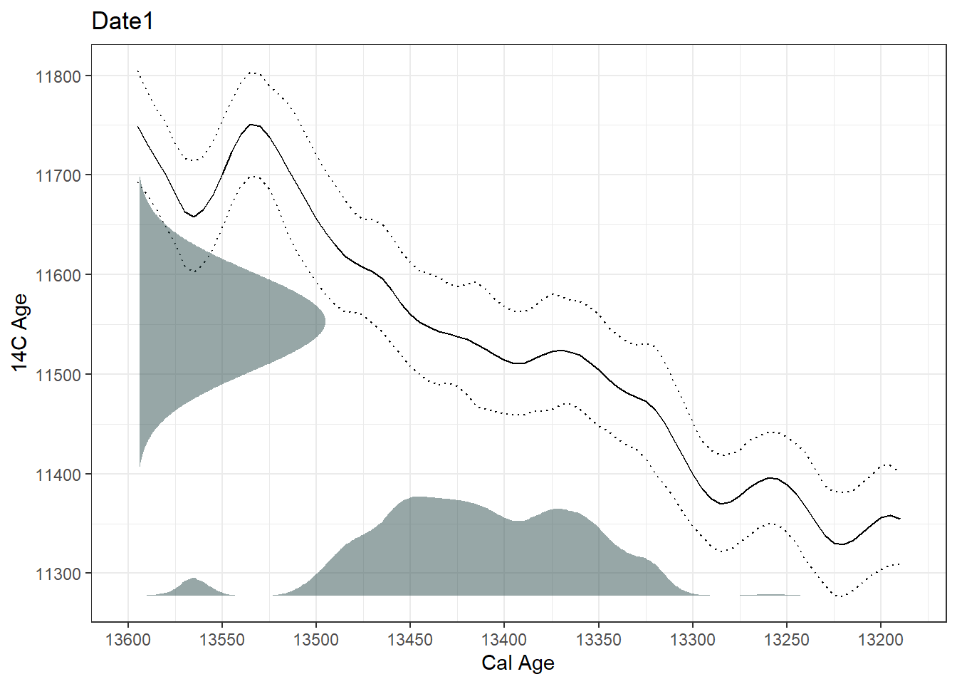
Notice that the calibrated distribution is not symmetrical, and not necessarily a single peak. Its shape is inherited from the wiggles in the curve, which is why a calibrated age can rarely be summarised honestly by one number.
Exercise 3.1
Using the code above, experiment with a few different ages and standard deviations. How does the shape of the calibrated distribution change with different ages and uncertainties?
Using the package documentation, find all the other possible
calCurvesarguments thatBchronaccepts.
3.2.1 Calibrating multiple radiocarbon dates
Here we’ll experiment with calibrating radiocarbon dates, using various calibration curves. Radiocarbon-dated samples come back from the lab with a radiocarbon age and standard deviation, among other information. These two bits of information are used to calibrate the radiocarbon dates to estimated ages. R packages may have useful vignettes (package tutorials) and built-in datasets that provide handy test templates. The following code is modified from the Bchron vignette.
ages <- BchronCalibrate(ages = c(3445, 11553, 7456),
                        ageSds = c(50, 230, 110),
calCurves = c('intcal20', 'intcal20', 'intcal20'))summary(ages)95% Highest density regions for Date1
$`94.4%`
[1] 3572 3834
95% Highest density regions for Date2
$`0.4%`
[1] 13004 13025
$`77.9%`
[1] 13059 13874
$`16.4%`
[1] 13923 14012
95% Highest density regions for Date3
$`94.6%`
[1] 8022 8423plot(ages)[[1]]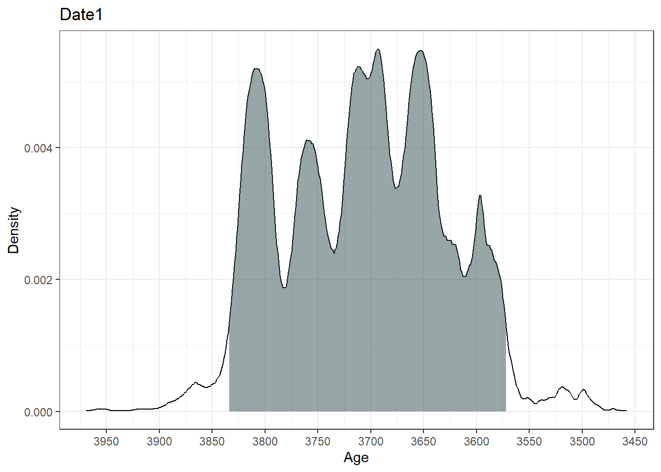
[[2]]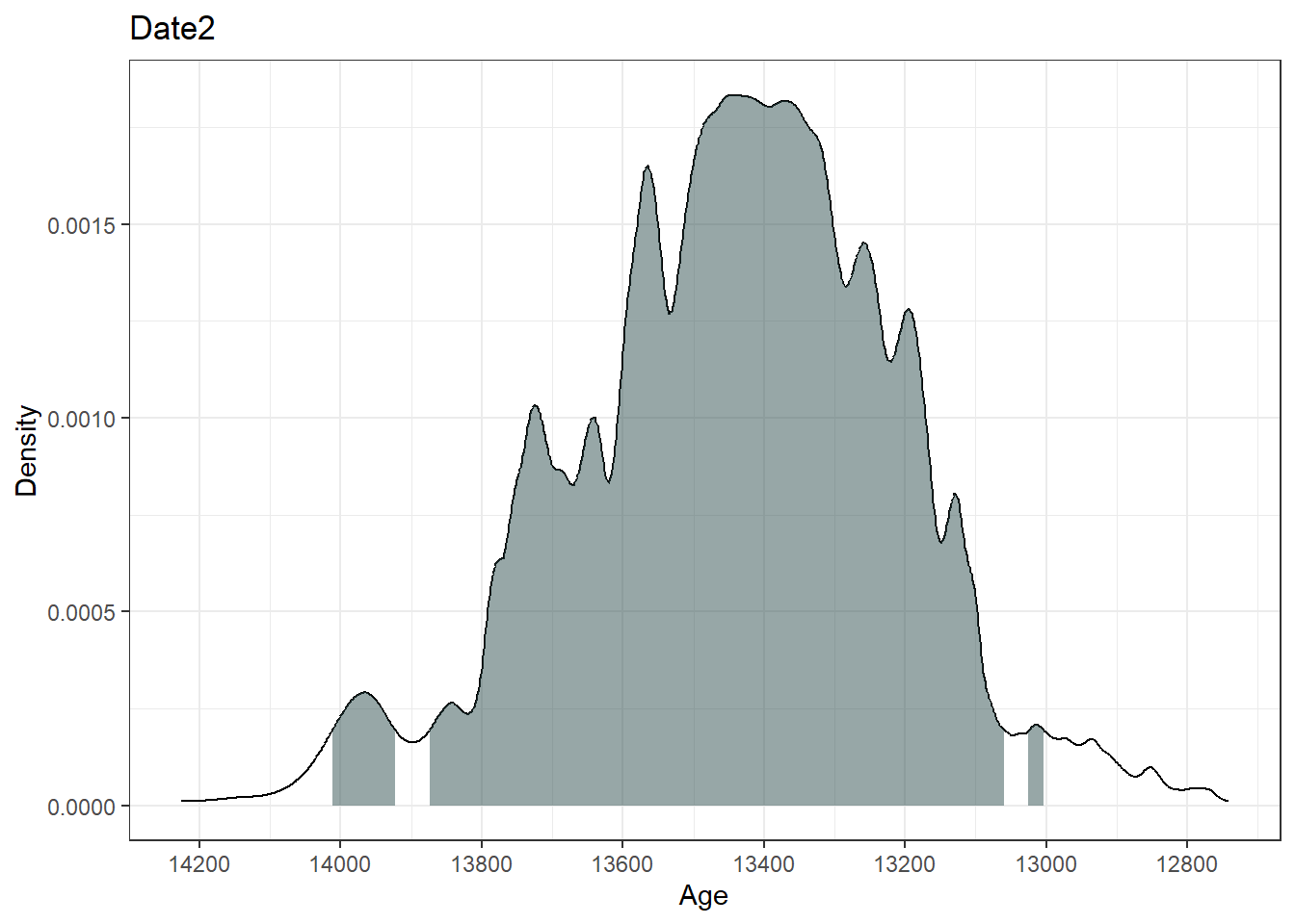
[[3]]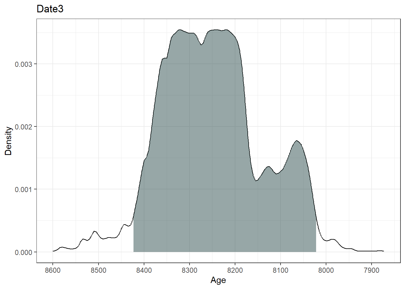
plot(ages, includeCal = TRUE, fillCol = 'red')`height` was translated to `width`.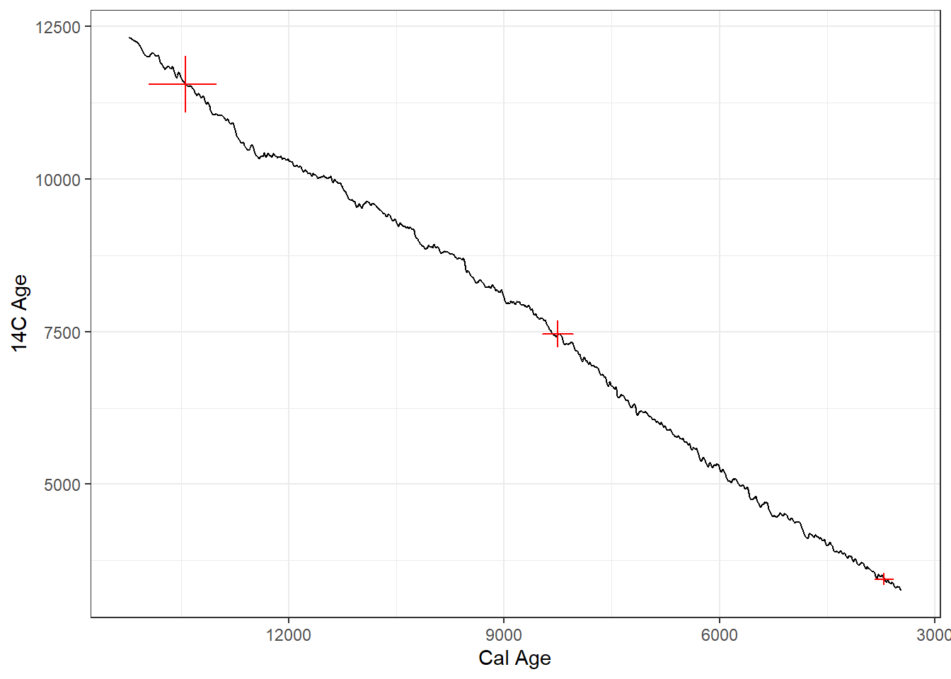
The output summary indicates the range of the highest density regions (i.e., the most likely ‘real’ age range of the sample). The plot function in Bchron outputs a ggplot object of the high density regions of the most likely ages.
The object you assigned the result of BchronCalibrate() to holds all of the calibration information, and it can be reached with $, for example ages$Date1$ageGrid.
Exercise 3.2 The three dates calibrated above were reported with standard deviations of 50, 230 and 110 radiocarbon years. Those numbers matter more than they look.
Recalibrate the same three ages, but set every
ageSdsto 30, roughly what a modern laboratory would report. Plot the result and compare it with the original. What happened to the shape of each distribution, and in particular to the number of separate peaks?Explain the change in terms of the calibration curve. It may help to plot a single date with
includeCal = TRUE, as in Figure 3.1.Now calibrate a single date of 8050 radiocarbon years with a standard deviation of 30, and look at what the calibration actually returns. The object holds two vectors of equal length, which you can see with
names():ageGrid, every calendar age the calibration considered, anddensities, how much probability sits at each of those ages.
Take the median of the grid alone, with
median(cal$ageGrid), and then work out the median of the distribution, which means finding the age at which the cumulative density first passes one half. Finally, runsummary()on the calibrated date and compare all three.The two medians will not agree, and neither of them will sit where you expect. Why not? What does
median(cal$ageGrid)actually measure? Look at how many separate regionssummary()reports and how much probability the largest of them carries, and then decide whether any single number would be an honest summary of this date.Finally, recalibrate one of your dates using the Southern Hemisphere curve (
shcal20) instead ofintcal20. How far does the estimated age move, and what would the consequence be of choosing the wrong one?
By the end of this exercise you should be able to look at a radiocarbon age, a standard deviation and a calibration curve, and say roughly what shape the calendar-age distribution will take and how confidently a single number could summarise it.
NoteMedian and mean ages
Commonly, only the median age is reported; however, it is good practice to report and consider the range of possible ages, especially when exploring synchroneity of events across space. Notice how Bchron focuses on delivering ranges and densities.
3.3 Types of age-depth model
Different kinds of age-depth models exist, each with their own underlying assumptions and behaviour. In the list below, #1-4 are classical or traditional forms of age-depth models, but Bayesian models are now the norm. The packages rbacon (usually referred to as ‘bacon’) and Bchron are the current standards for Bayesian age-depth modelling. Before going to Bayesian models, we’ll begin with the classics.
Linear interpolation, a.k.a. ‘connect the dots,’ in which straight lines are drawn between each depth-adjacent pair of age controls.
Linear regression (\(y = b_0 + b_1 x\), where \(y\) is age, \(x\) is depth, and \(b_0\) and \(b_1\) are constants), in which a single straight line is fitted through the entire set of age controls. In ordinary least squares (OLS), the chosen line is the one that minimises the sum of the squared vertical distances between the points and the line. Standard OLS assumes that all observations are normally distributed, which is a poor assumption for calibrated radiocarbon dates.
Polynomials, also fitted to the entire set of age controls (\(y = b_0 + b_1 x + b_2 x^2 + b_3 x^3 + \dots + b_n x^n\)), are an extension of linear regression, with additional terms for \(x^2\), \(x^3\), etc. Some arbitrary maximum \(n\) is chosen, usually in the range of 3 to 5. These are called ‘third-order polynomials,’ ‘fifth-order polynomials,’ etc.
Splines, which are a special kind of polynomial function, locally fitted to subsets of the age controls and then smoothly interpolated between points. (Several different formulas can be used to generate splines; common forms include cubic, smoothing and monotonic splines. LOWESS is often used for the same purpose but is a local regression smoother rather than a spline.)
Bayesian age models (e.g.,
bacon,bchron,oxcal, etc.). Bayesian models differ in detail, but all combine a statistical representation of prior knowledge with the new data (i.e. the age controls at a site) to build an age-depth model with posterior estimates of age for any given depth. Bayesian models are now widely used because:- they allow the incorporation of prior knowledge (e.g., from coring many lakes, we now have decent estimates of typical sediment accumulation rates, see Goring et al. (2012))
- they can handle highly irregular probability distribution functions such as those for radiocarbon dates after calibration; and as a result
- they generally do a better job of describing uncertainty than traditional age-depth models
3.3.1 Classical age-depth models
Classical models are now out-dated methods (Blaauw et al. 2018), but it is useful to understand how they work, because the literature published before the relatively recent development of Bayesian methods relies on them. Let’s explore some classical methods of age-depth modelling using one of the datasets included with the Bchron package. The data are from a core at Sluggan Moss in County Antrim, Northern Ireland. The published record calls the site Sluggan Bog (Smith and Goddard 1991); both names refer to the same place, and Bchron uses both in its own documentation. The dataset is called via:
data(Sluggan) # Call the data from Bchron
head(Sluggan) # Check out the data
id ages ageSds position thickness calCurves
1 UB-201A 985 45 44.5 5 intcal20
2 UB-211A 1225 65 49.5 5 intcal20
3 UB-437 1635 75 69.0 2 intcal20
4 UB-748 2130 45 102.0 4 intcal20
5 UB-438 2930 85 125.0 2 intcal20
6 UB-439 3945 85 165.0 2 intcal20Notice that some depths appear more than once. Sluggan Moss was dated in replicate at several levels, with three separate radiocarbon determinations at 272.5 cm and at 367.5 cm, for instance. Replicate dating is good practice, because it shows how reproducible a determination is, but it does mean the classical methods below have to decide what to do when one depth carries several ages.
Linear interpolation predicts ages by simply drawing a line between successive dated samples. This method assumes that there is a constant age-depth relationship between samples, an assumption that is unlikely to be true, especially for cores with fewer dated samples than Sluggan Moss.
# Interpolate an age for every depth. ties = mean averages the replicate dates at
# those depths that were dated more than once.
interp_ages <- approx(x = Sluggan$position, y = Sluggan$ages, ties = mean)

# Age on the horizontal axis, depth on the vertical and increasing downwards
plot(x = interp_ages$y, y = interp_ages$x, type = "l",
     xlab = "Age (14C years BP)", ylab = "Depth (cm)",
     ylim = rev(range(Sluggan$position)))
points(x = Sluggan$ages, y = Sluggan$position, cex = 1.5, col = "red")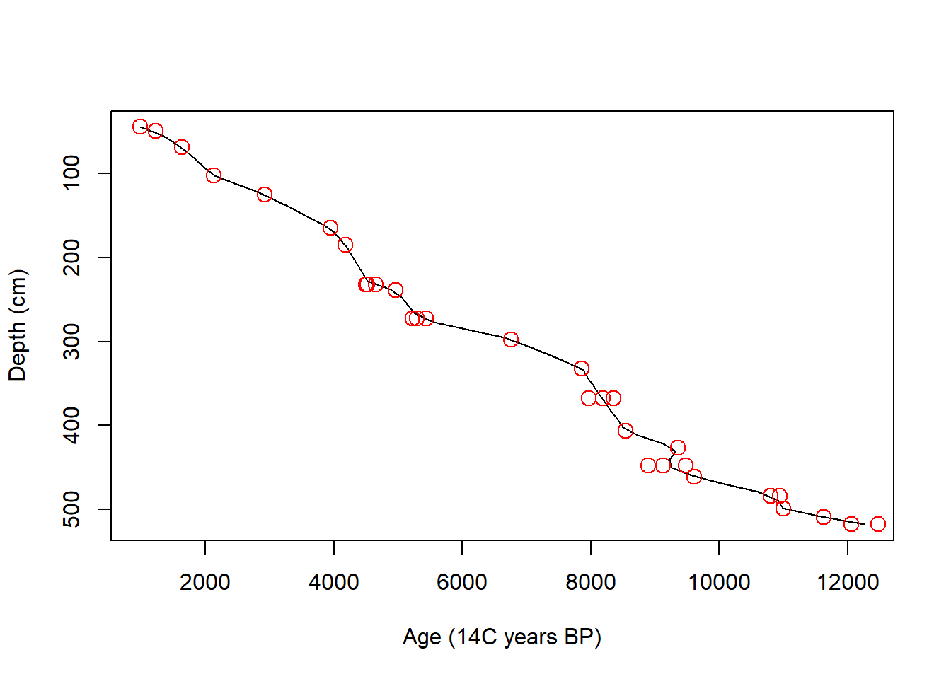
Linear regression provides a line of best fit through the dated samples. This method assumes a constant age-depth relationship across all samples, also unlikely to be true depending on processes affecting the core during its formation.
mod_ages <- lm(ages ~ position, data = Sluggan) # age as a function of depth

# A grid of depths to predict ages at, used by this model and the two below
depth_grid <- seq(from = min(Sluggan$position), to = max(Sluggan$position),
                  length.out = 250)

plot(x = Sluggan$ages, y = Sluggan$position, cex = 1.5, col = "red",
     xlab = "Age (14C years BP)", ylab = "Depth (cm)",
     ylim = rev(range(Sluggan$position)))
lines(x = predict(mod_ages, data.frame(position = depth_grid)), y = depth_grid)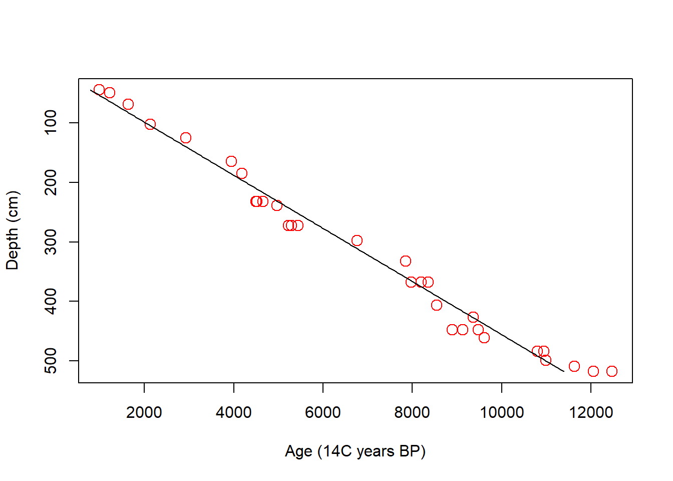
Polynomial regression allows a curve to be fit through the data. The amount the curve ‘wiggles’ depends on the order of the polynomial fit to the data. Polynomial regression runs the risk of over-fitting.
poly_ages <- lm(ages ~ poly(position, 3), data = Sluggan)

plot(x = Sluggan$ages, y = Sluggan$position, cex = 1.5, col = "red",
     xlab = "Age (14C years BP)", ylab = "Depth (cm)",
     ylim = rev(range(Sluggan$position)))
lines(x = predict(poly_ages, data.frame(position = depth_grid)), y = depth_grid)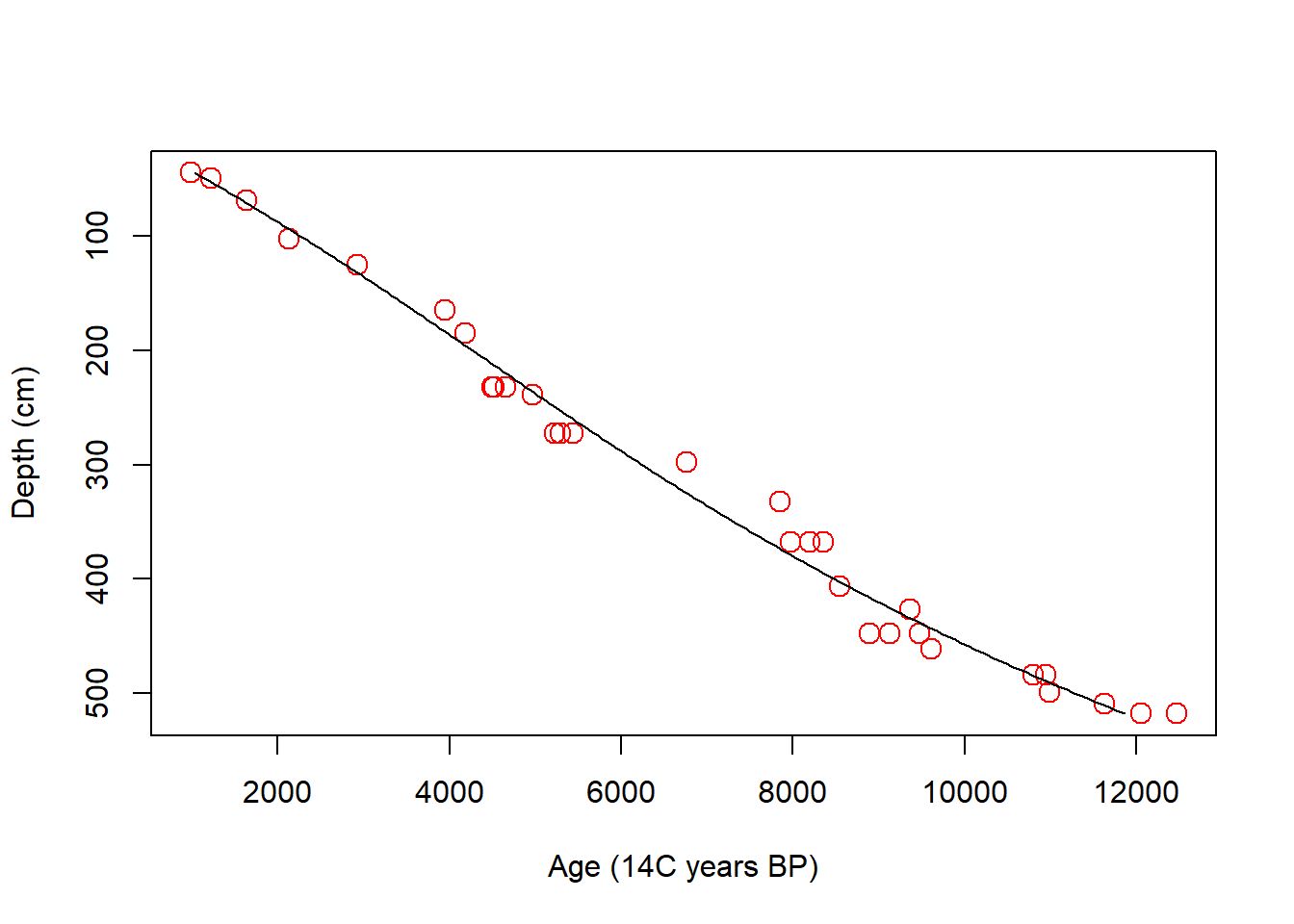
Splines are a class of functions including, for example, smoothing splines and cubic splines. Cubic splines are piece-wise polynomials fitted locally between ‘knots’. That is, the data are split into bins, and a separate polynomial is fitted within each bin, with the pieces joined smoothly at the knots. By default the bs() function uses a third-degree polynomial, so without any knots the fit looks the same as the third-order polynomial above. Note that the knots are positions along the predictor, so here they are depths in centimetres.
cubic_ages <- lm(ages ~ splines::bs(position, knots = c(100, 250, 400)),
                 data = Sluggan)

plot(x = Sluggan$ages, y = Sluggan$position, cex = 1.5, col = "red",
     xlab = "Age (14C years BP)", ylab = "Depth (cm)",
     ylim = rev(range(Sluggan$position)))
lines(x = predict(cubic_ages, data.frame(position = depth_grid)), y = depth_grid)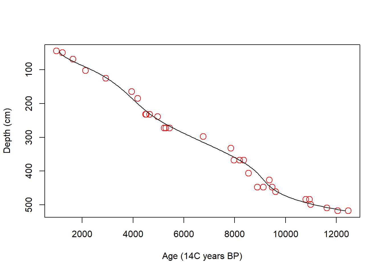
Because classical age-depth modelling is rarely used now, we are not going to delve further into the statistical details of the best way of fitting each model (e.g., the number of knots to use for fitting a cubic spline).
3.3.2 Bayesian age-depth models
Now let’s see what the latest methods show for the same dataset.
Note that all the values provided to the arguments are contained in the Sluggan dataframe. When creating chronologies from your own (or accessed) data, you may need to rename them to match your data.
set.seed(1984) # the model is stochastic, so fix the seed for reproducibility

SlugganOut <- with(Sluggan,
                   Bchronology(ages = ages,
                               ageSds = ageSds,
                               calCurves = calCurves,
                               positions = position,
                               positionThicknesses = thickness,
                               ids = id,
                               predictPositions = seq(min(Sluggan$position),
                                                      max(Sluggan$position),
                                                      by = 10)))
The summary shows for each position (depth) the median and quartiles of the predicted ages for that position.
summary(SlugganOut)Quantiles of predicted ages by depth:
Depth 2.5% 25% 50% 75% 97.5%
44.5 649.900 826.00 887.0 938.00 1045.150
54.5 1073.975 1183.00 1242.0 1302.00 1432.025
64.5 1219.000 1348.00 1408.0 1474.00 1597.025
74.5 1453.000 1572.00 1644.0 1733.00 1935.050
84.5 1546.875 1728.75 1818.5 1917.25 2093.100
94.5 1714.000 1898.75 1982.5 2062.00 2219.025
104.5 2077.000 2180.00 2281.0 2372.00 2705.000
114.5 2260.975 2508.75 2639.0 2778.25 3024.050
124.5 2739.900 2952.00 3037.0 3128.25 3314.050
134.5 3062.950 3271.00 3408.0 3571.25 3923.025
144.5 3227.950 3542.00 3696.5 3864.00 4193.075
154.5 3459.000 3814.00 3973.0 4117.25 4338.050
164.5 3983.950 4190.75 4282.0 4381.50 4506.025
174.5 4267.950 4411.75 4491.0 4558.00 4690.000
184.5 4437.975 4577.00 4647.0 4721.00 4831.000
194.5 4560.975 4695.00 4774.5 4847.00 4975.050
204.5 4615.800 4781.75 4854.5 4930.00 5083.025
214.5 4691.925 4864.00 4943.5 5013.25 5139.075
224.5 4814.925 4960.75 5031.0 5093.25 5226.000
234.5 5220.975 5345.00 5425.0 5477.25 5581.025
244.5 5612.000 5689.00 5741.0 5796.00 5925.025
254.5 5684.975 5779.75 5836.5 5893.00 6003.050
264.5 5747.950 5873.00 5927.0 5975.00 6070.075
274.5 6096.975 6223.00 6281.0 6361.00 6767.150
284.5 6401.000 6685.75 6864.0 7050.25 7382.125
294.5 6772.000 7243.00 7406.5 7501.00 7635.025
304.5 7563.950 7722.75 7817.5 7947.25 8264.150
314.5 7705.950 7940.75 8088.0 8231.25 8535.025
324.5 7916.825 8203.75 8344.5 8457.00 8678.125
334.5 8430.000 8545.50 8624.0 8719.00 8907.025
344.5 8514.975 8654.75 8745.5 8832.50 9012.025
354.5 8592.975 8748.00 8843.0 8930.00 9080.100
364.5 8690.925 8860.00 8971.0 9036.25 9160.075
374.5 9140.875 9276.00 9342.5 9426.25 9566.075
384.5 9222.950 9356.00 9429.0 9508.00 9715.050
394.5 9293.975 9431.00 9501.5 9595.25 9831.100
404.5 9377.925 9510.00 9593.0 9707.00 9971.000
414.5 9568.950 9737.00 9860.0 9978.50 10193.025
424.5 9701.825 9940.00 10124.0 10214.00 10341.175
434.5 9896.950 10107.00 10286.0 10347.00 10527.025
444.5 10009.900 10229.75 10341.0 10415.00 10612.175
454.5 10562.000 10742.00 10834.0 10936.00 11131.075
464.5 10999.975 11220.75 11347.5 11548.25 12117.325
474.5 11315.000 11801.00 12009.5 12218.25 12542.075
484.5 12402.925 12674.00 12759.0 12838.25 12995.050
494.5 12807.000 12919.75 12979.5 13040.00 13164.025
504.5 13069.925 13220.00 13309.5 13389.00 13578.000
514.5 13541.000 13760.00 13865.0 13970.50 14194.150Bchron estimates, for each date, the probability that it is an outlier given all of the others. A high value flags a date that disagrees with its neighbours.
summary(SlugganOut, type = "outliers")Posterior outlier probability by date:
Date OutlierProb
UB-201A 0.011
UB-211A 0.006
UB-437 0.008
UB-748 0.009
UB-438 0.010
UB-439 0.007
UB-440 0.008
UB-219D 0.004
UB-219B 0.014
UB-219A 0.009
UB-441 0.013
UB-220D 0.048
UB-220A 0.015
UB-220E 0.016
UB-221A 0.010
UB-749 0.009
UB-223B 0.161
UB-223A 0.012
UB-223D 0.131
UB-442 0.009
UB-443 0.055
UB-225B 0.227
UB-225D 0.016
UB-225F 0.017
UB-444 0.009
UB-227D 0.006
UB-227F 0.011
UB-446 0.007
UB-447 0.011
UB-229D 0.013
UB-229F 0.054plot(SlugganOut)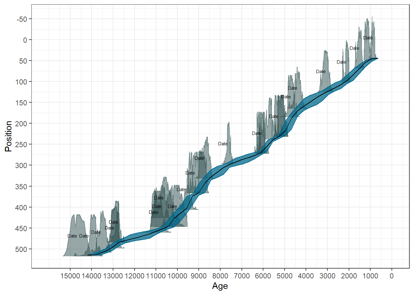
A more complete version of the modelling process using Bchron can be found in the vignette.
Exercise 3.3 Sluggan Moss is particularly well dated, with 31 age controls. This exercise asks what you lose as dated intervals are removed. For example, a core may only have 5 or 10 dated samples, how would this change your confidence in the age-depth model output, and importantly, your subsequent ecological inferences?
Build several down-sampled versions of the
Sluggandata at different resolutions, for example by keeping every second control, then every fourth, then only five or six spread through the core. Always keep the first and last control, so that every version spans the same depth range and none of the models has to extrapolate.Fit a
Bchronology()model to each version, rememberingset.seed()so your results are reproducible, and plot them.Compare the shape of the age-depth relationship and the width of the uncertainty band. Where in each core is the model most confident, and where is it least? What happens to the uncertainty in the gaps as the gaps get longer?
If you were planning a coring campaign with a fixed budget for radiocarbon dates, what would these results tell you about where to place them?
TipResources
Age-depth modelling is complicated: there are many pitfalls, assumptions, and uncertainties that are often ignored. Recent developments have begun to focus on quantifying uncertainties to understand the reliability of inferences made from the data. Key papers for understanding age-depth modelling include:
3.4 Accumulation rate
Having a chronology is not the end of it. Because the model gives an age at every depth, it also tells us how fast sediment accumulated, which is simply the rate of change of age with depth. Bchron will return that directly, as a distribution rather than a single line:
acc_rate <- summary(SlugganOut,
                    type = "acc_rate",
probs = c(0.25, 0.5, 0.75))ggplot(acc_rate, aes(x = age_grid, y = `50%`, ymax = `75%`, ymin = `25%`)) +
geom_line() +
geom_ribbon(alpha = 0.2) +
scale_x_reverse() +
labs(y = "Accumulation rate (cm per year)",
x = "Age (cal years BP)") +
theme_bw()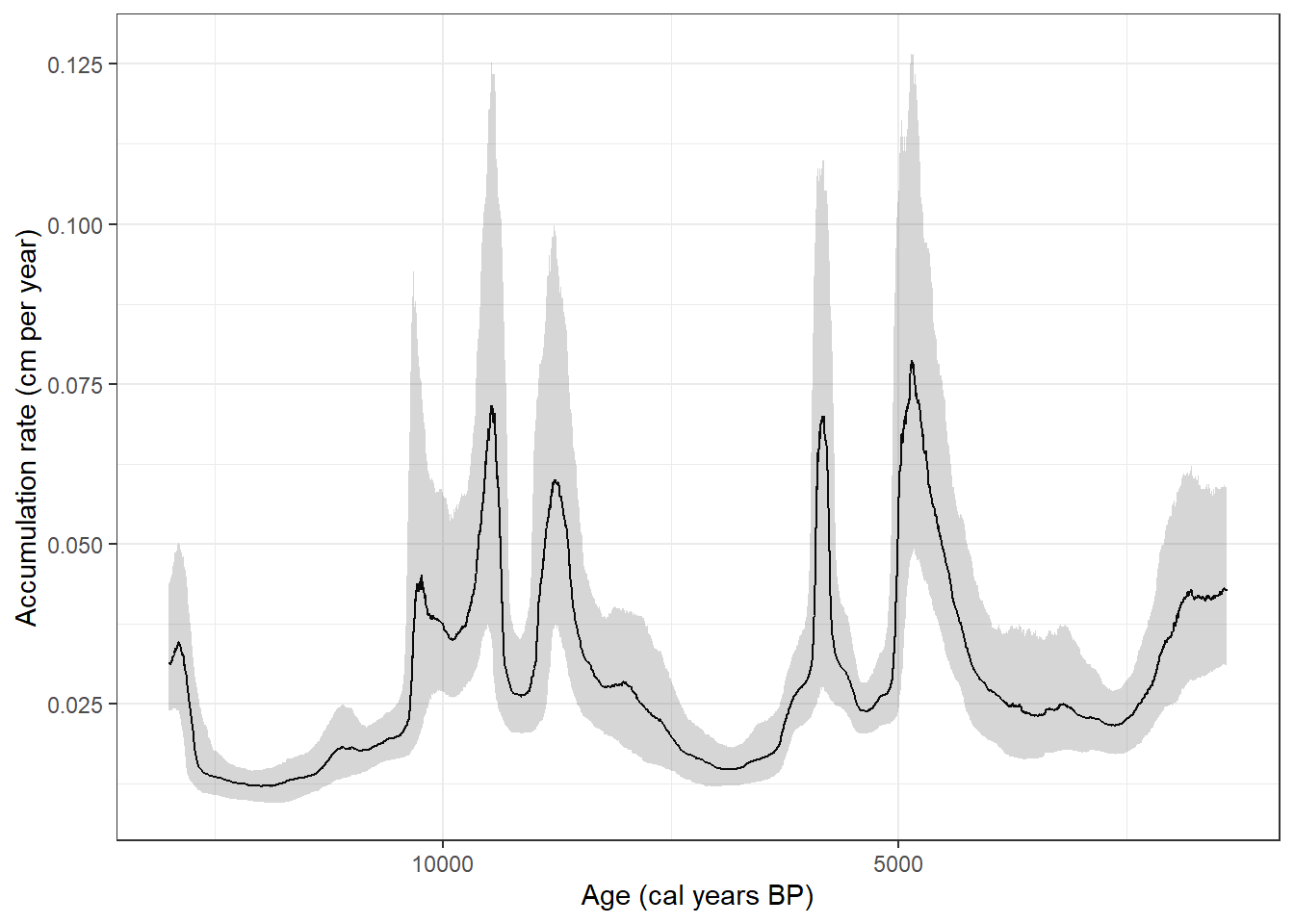
Two things are worth drawing out of Figure 3.8. Accumulation rate is a derivative of the age-depth model, so it inherits all of that model’s uncertainty and amplifies it; the ribbon here is an interquartile range, not a measurement error. And the rate is not constant, which is precisely the assumption that linear interpolation and linear regression were making earlier in this chapter. Sediment does not accumulate at a steady pace, and a chronology that pretends otherwise will misdate everything between its control points.
3.5 Rebuilding chronologies in Neotoma
So far we have used a dataset built into Bchron. If you are using data from Neotoma, you will be downloading and working with data that may have their own chronologies associated with them. Many archived chronologies predate the Bayesian methods, or use older calibration curves, so it may be best to rebuild them with the latest methods. Such a chronology is not wrong so much as superseded, and any re-analysis that inherits it inherits its assumptions too. Checking, and often rebuilding, the chronology is a routine and important part of working with archived data.
We obtained data from Neotoma with the neotoma2 package in Chapter 2, so the downloading here will look familiar; the only new part is what we do with the chronological controls once we have them. As before we save each download rather than repeating it.
if (!file.exists("./data/devils_dl.rds")) {
  devils_dl <- neotoma2::get_sites(siteid = 666) %>%
    neotoma2::get_datasets(all_data = TRUE) %>%
    neotoma2::filter(datasettype == "pollen") %>%
    neotoma2::get_downloads()
  saveRDS(devils_dl, "./data/devils_dl.rds")
} else {
  devils_dl <- readRDS("./data/devils_dl.rds")
}
The chronological controls are the dates and other markers the original authors used. A core may carry more than one chronology, so the first thing to ask is how many there are:
controls <- neotoma2::chroncontrols(devils_dl)

unique(controls$chronologyid)
[1] 310 9930 23996
NoteMultiple chronologies! 🧙
Note that Devil’s Lake has three different chronologies, not one. If you take the first that comes back, or assume there is only ever one, you may be working with a chronology that its own authors superseded. They are not interchangeable: these three contain 11, 13 and 13 controls respectively, and they do not use the same kinds of control as each other.
Sites may also get revisited, and new dates get added to the database. Always look at what is available, and be able to say why you chose the one you did. Where publications are listed alongside a chronology, use them for reference.
We will use chronology 9930. Note what its controls are made of:
controls <- neotoma2::chroncontrols(devils_dl) %>%
  dplyr::filter(chronologyid == 9930) %>%
  dplyr::arrange(depth)

controls[, c("chroncontrolid", "depth", "thickness",
             "chroncontrolage", "chroncontroltype")]
chroncontrolid depth thickness chroncontrolage chroncontroltype
1 38069 0.00 1.0 0 Core top
2 38070 21.50 7.0 120 Ambrosia rise
3 38058 151.50 5.0 2055 Radiocarbon
4 38059 166.50 5.0 2430 Radiocarbon
5 38060 265.00 4.0 4105 Radiocarbon
6 38061 336.00 4.0 5245 Radiocarbon
7 38062 397.00 4.0 6920 Radiocarbon
8 38063 457.00 4.0 8640 Radiocarbon
9 38064 474.00 2.0 8590 Radiocarbon
10 38065 535.00 1.0 9740 Radiocarbon
11 38066 550.00 2.0 10110 Radiocarbon
12 38067 583.75 2.5 10730 Radiocarbon
13 38068 633.00 12.0 12580 RadiocarbonOnly eleven of the thirteen are radiocarbon dates. There is a core top, taken as the year of extraction, and there is an Ambrosia rise, the pollen marker for EuroAmerican land clearance mentioned at the start of this chapter. Both are already calendar ages. They must not be calibrated, and this is exactly the distinction the calCurves argument exists to make.
The controls dataframe holds nearly everything Bchronology() needs, but not in the same shape as the Sluggan data. Sluggan has a single standard deviation per date; Neotoma stores an older and a younger limit, so the standard deviation is the distance from the age to either limit. And there is no calibration curve column at all, so we build one from the control type:
controls <- controls %>%
  dplyr::mutate(
    ageSds    = abs(agelimityounger - chroncontrolage),
    calCurves = ifelse(chroncontroltype == "Radiocarbon", "intcal20", "normal"))

controls[, c("depth", "chroncontrolage", "ageSds", "chroncontroltype", "calCurves")]
depth chroncontrolage ageSds chroncontroltype calCurves
1 0.00 0 10 Core top normal
2 21.50 120 10 Ambrosia rise normal
3 151.50 2055 65 Radiocarbon intcal20
4 166.50 2430 65 Radiocarbon intcal20
5 265.00 4105 65 Radiocarbon intcal20
6 336.00 5245 65 Radiocarbon intcal20
7 397.00 6920 75 Radiocarbon intcal20
8 457.00 8640 85 Radiocarbon intcal20
9 474.00 8590 50 Radiocarbon intcal20
10 535.00 9740 50 Radiocarbon intcal20
11 550.00 10110 140 Radiocarbon intcal20
12 583.75 10730 50 Radiocarbon intcal20
13 633.00 12580 130 Radiocarbon intcal20Devil’s Lake is in Wisconsin, so the radiocarbon dates get intcal20. A southern-hemisphere core would need shcal20, and a marine record marine20. Everything that is not a radiocarbon date gets normal, meaning “treat this age as it stands”. Deriving the vector rather than typing it out means it stays correct if the chronology changes.
set.seed(1984)

newChron <- Bchron::Bchronology(
  ages                = controls$chroncontrolage,
  ageSds              = controls$ageSds,
  calCurves           = controls$calCurves,
  positions           = controls$depth,
  positionThicknesses = controls$thickness,
  ids                 = controls$chroncontrolid,
predictPositions = seq(min(controls$depth), max(controls$depth), by = 10))plot(newChron)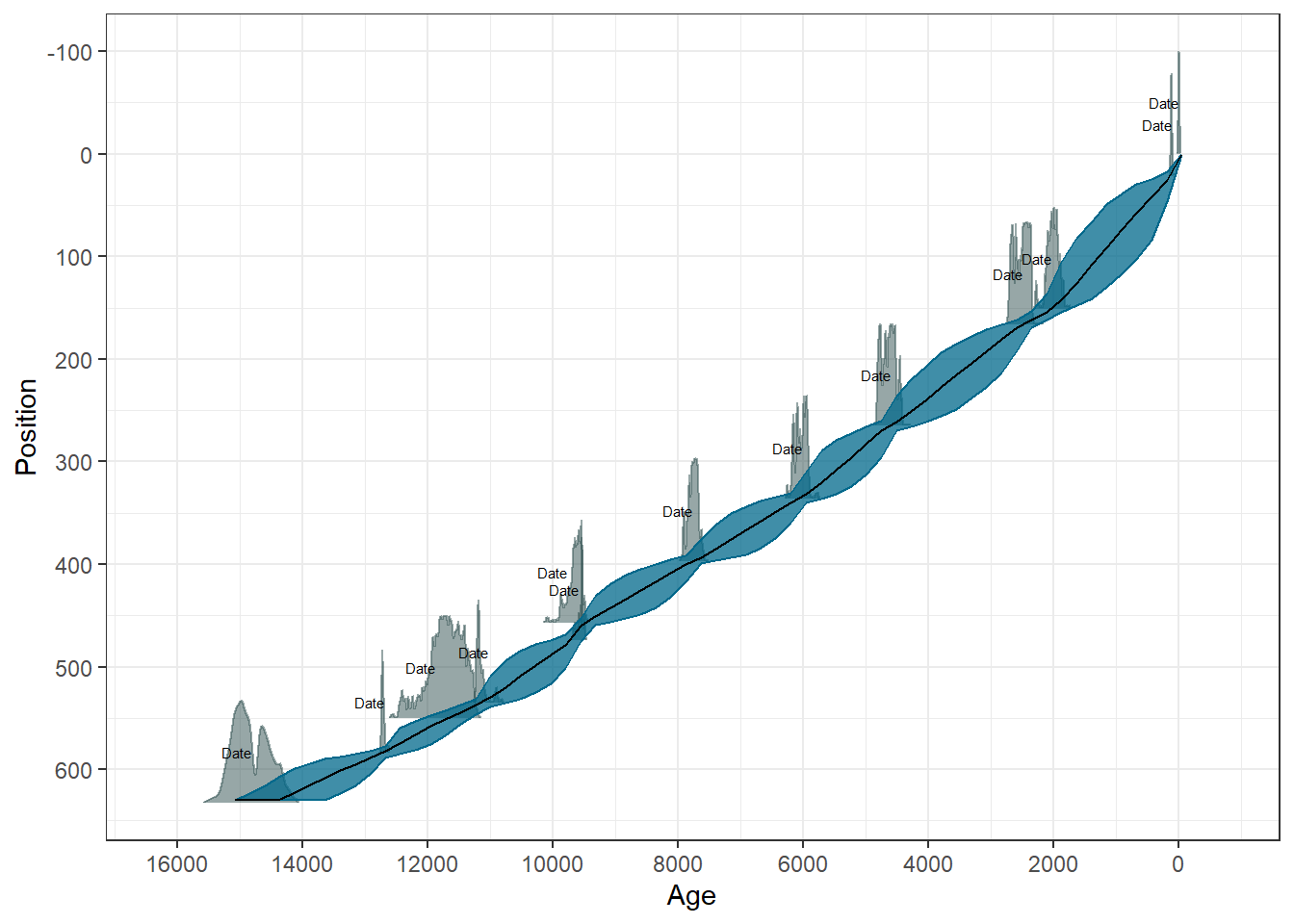
Look closely at the two controls at 457 and 474 cm. The deeper of the two is reported as the younger, 8590 against 8640 radiocarbon years, which cannot be true of undisturbed sediment. The outlier probabilities pick this up:
summary(newChron, type = "outliers")Posterior outlier probability by date:
Date OutlierProb
38069 0.009
38070 0.009
38058 0.007
38059 0.007
38060 0.006
38061 0.007
38062 0.007
38063 0.027
38064 0.032
38065 0.008
38066 0.006
38067 0.006
38068 0.013Those two dates carry the highest outlier probabilities of the thirteen, several times the value of any other. They are still low in absolute terms, because the two ages agree well within their uncertainties, but the model has noticed. This is the advantage of a method that carries uncertainty explicitly: it can register that something is odd without being derailed by it, where a classical fit would simply have drawn a line through the inversion.
We have downloaded a range of sites from the northern and southern hemispheres, for you to use in the following exercise. If you prefer, you can also choose a site of your own using neotoma2 or Neotoma Explorer.
if (!file.exists("./data/some_sites.rds")) {
  site_ids <- c(10063, 1639, 10136, 28408, 9865, 28489, 31732, 666, 27671)
  some_sites <- neotoma2::get_sites(site_ids)
  saveRDS(some_sites, "./data/some_sites.rds")
} else {
  some_sites <- readRDS("./data/some_sites.rds")
}

neotoma2::plotLeaflet(some_sites)
Exercise 3.4 Rebuild a chronology for a site of your own choosing, and get the calibration curve vector right.
Pick a site (not Devil’s Lake,
ID = 666) either from the ones given above, or any of your choosing!List the available chronologies and choose one, saying why.
Work out what kind each chronological control is, and build a
calCurvesvector accordingly. Remember that the hemisphere decides betweenintcal20andshcal20, and that anything already expressed as a calendar age needsnormal.Fit the model and plot it. Compare the uncertainty with the published chronology if the original paper is available.
Not every site will cooperate. If Bchronology() refuses to run, read the error: it is usually telling you that a control is missing something it needs. Deciding what to do about a control with no reported uncertainty is part of the work, not a distraction from it.
3.6 Conclusion
We have calibrated radiocarbon dates and seen how much uncertainty that conversion adds, fitted the four classical age-depth models and seen where each of them misleads, and built a Bayesian chronology that carries its uncertainty through to every predicted age. Chronologies underpin inferences made from statistical analyses, and are thus a crucial part of the analytical process. Age-depth models are often used to determine the timing of biological events, and accumulation rates affect how many years of ecological productivity are contained within a given sample (known as time averaging).
The exercises are linked below if you need to revisit them:
- Exercise 3.1, reading a single date against the curve
- Exercise 3.2, what a standard deviation does to a calibrated age
- Exercise 3.3, and what happens to a chronology as its dates thin out
- Exercise 3.4, rebuilding a published chronology yourself