The modern analog technique (MAT) is a standard approach for making quantitative inferences about past vegetation and climate from fossil pollen data – and from many other forms of paleoecological data (Chevalier et al. 2020; J. W. Williams and Shuman 2008; Gavin et al. 2003; Overpeck, Webb, and Prentice 1985). The MAT relies on reasoning by analogy (Jackson and Williams 2004), in which it is assumed that two compositionally similar pollen assemblages were produced by similar plant communities, growing under similar environments. The similarity of pollen assemblages is determined by the calculation of dissimilarity metrics.
The MAT can also be thought of as a non-parametric statistical technique, that computer scientists call a \(k\)-nearest neighbors algorithm. It is a simple form of machine learning. Each fossil pollen assemblage is matched to 1 or more (\(k\)) modern pollen assemblages, then is assigned the ecological and environmental characteristics associated with those modern analogues.
The MAT is a popular approach for reconstructing past environments and climates, due to its relative simplicity and intuitive appeal. However, like any algorithm, if used unwisely, it can produce spurious results. More generally, when reasoning by analogy, be careful! Analogies are always incomplete and imperfect, and you must use your critical judgment to determine whether these imperfections are minor or serious.
To reconstruct past environments using the MAT, we need three data sets:
Modern species assemblages.
Modern environmental variables.
Fossil species assemblages.
The MAT follows four basic steps:
Calculate dissimilarities between a fossil species assemblage \(i\) and all modern species assemblages in set \(S\).
Discard modern samples with dissimilarities greater than a threshold threshold.
Identify and retain the \(k\) closest modern analogs.
Average the environmental conditions associated with the modern analogs and assign them to fossil sample \(i\).
Note that we are taking a detour into paleoclimatology for two reasons. First, because paleoclimatic reconstructions are still a primary use for fossil pollen and other micropaleontological data. Second, because the MAT and the analogue package, as a dissimilarity-based approach, also lets us explore the novelty of past communities - perhaps of more interest to paleoecologists than inferred paleoclimates!
The following section, Section 7.2.1, takes you through some pretty advanced data wrangling required to match species names between the datasets we will use. However, if you prefer to skip all the wrangling and jump directly to the anayses in Section 7.2.2, the data have been saved post-wrangling and can be loaded into R directly. Run the ‘Jump point’ code below and portal to Section 7.2.2.
Jump point
Run this code (unfold the code chunk below) to load in the pre-wranged data and portal to Section 7.2.2
In this case, data are coming from two separate sources, NeotomaDB and the North American Modern Pollen Dataset (NAMPD). We will use the NAMPD (Whitmore et al. 2005) for the cross-validation analysis. Note that the NAMPD is pre-loaded into the analogue package, but here we’ll use use the original (more complete) data so that we can filter locations easily. Some of the data wrangling required to get two matrices containing the same species with identical names for the correct region (as required by the MAT function) is fairly advanced. This type of wrangling is quite common in palaeoecological data-science as you may be dealing with, for example, raw data collected by individuals, or from different databases that are stored in inconsistent formats.
Ready to Wrange? Let’s get the data ready:
Packages required for this section
# Load up the packagesif (!require("pacman")) install.packages("pacman", repos="http://cran.r-project.org")pacman::p_load(neotoma2, tidyverse, neotoma2, analogue, vegan, readxl, fuzzyjoin)
Respawn point
The following code (unfold by clicking the dropdown) downloads the data from the neotoma API and formats it with basic harmonisation and pollen proportions calculated. This part of the data wrangling is covered in detail in Chapter 4 so, more easily, you can read in the pre-wrangled .rds file from the data directory. Note that this is the long format data not the species only matrix from the jump point above.
Code
# The following code can be done in one pipeline but we have split it into chunks to help with readablitydevils_samples <-get_sites(siteid =666) %>%# Download the site samples dataget_downloads() %>%samples()devils_samples <- devils_samples %>% dplyr::filter(ecologicalgroup %in%c("UPHE", "TRSH"), # Filter ecological groups by upland heath and trees and shrubs elementtype =="pollen", # filter bu pollen samples units =="NISP") %>%# Filter by sampling unitmutate(variablename =replace(variablename, stringr::str_detect(variablename, "Pinus.*"), # Harmonize Pinus into one group"Pinus"),variablename =replace(variablename, stringr::str_detect(variablename, "Ambrosia.*"),"Ambrosia")) %>%group_by(siteid, sitename, sampleid, variablename, units, age, agetype, depth, datasetid, long, lat) %>%summarise(value =sum(value), .groups='keep') # The group_by function will drop columns not used as grouping variablesdevils_samples <- devils_samples %>%# Calculate proportions of each species by year groupgroup_by(age) %>%mutate(pollencount =sum(value, na.rm =TRUE)) %>%group_by(variablename) %>%mutate(prop = value / pollencount) %>%arrange(desc(age)) %>%ungroup()# saveRDS(devils_samples, "./data/devils_samples.rds") # Save the data for later
To read in the pre-wrangled long data for Devil’s Lake use:
# Load up the datadevils_samples <-readRDS("./data/devils_samples.rds")
We will use the North American Modern Pollen Database (NAMPD) to create modern analogues. The NAMPD includes both modern surface pollen samples, and climate measurements. The NAMPD is not (yet) accessible through neotoma but is stored on servers at the University of Madison, WI. JACK ACTION POINT: to use this method in other regions what databases are available? The following code does not need to be run but shows how to download the NAMPD from the server to your data directory and unzip the downloaded data from R.
Since the data are already saved in the data directory, let’s read it in from there. The step of downloading data might often be done manually, the point of including the R code is to maintain a reproducible work-flow. It is always good to keep your own copy of the data just in case. Servers may not be maintained forever, or data may be removed for example.
Still with me? Great! Now we have our three datasets:
Our site of interest (Devil’s Lake palaeo data).
Our modern pollen data.
Our modern climate measurements.
The modern datasets includes the whole of North America and need to be filtered for the Eastern US so that the taxa are relevant to the those in Devil’s Lake. We’re first going to filter by longitude, then select by taxa so that we have a matching matrix of species between Devil’s Lake palaeo-data and the modern surface samples from the NAMPD. We are going to keep all data East of 105°W, see Krause et al. (2019) and John W. Williams, Shuman, and Webb III (2001).
# several columns contain data not used for the MATmod_pol_east <- mod_pol %>%filter(LONDD >=-105) %>%# Filter for sites east of -105 degreesselect(ID2, 14:147) # Select colums with ID and species only# Many functions require site-by-species matrices in wide format# Note we pivoted by age so we have an age column not used in MATdevils_wide <- devils_samples %>%pivot_wider(id_cols = age, names_from = variablename, values_from = prop) %>%replace(is.na(.), 0)# Store ages separately for plotting later:devils_ages <- devils_wide$age
We will also filter the modern climate records by the same ID to match the modern pollen records.
Right, now is the tricky part of matching species names. Unfortunately, the species names between data downloaded from Neotoma and the NAMPD do not match exactly. Sometimes matching is easiest done manually but because of the number of species in both datasets we will do as much as possible programatically. The fuzzyjoin package allows us to match strings (names) by a distance measure and outputs a number of possible matches.
looks like it’s done a good job for the most part! Butthere are a few mismatches.
# Save the names of each dataset and convert all to lowercasemod_pol_names <-as_tibble(tolower(colnames(mod_pol_east[-1])))devil_names <-as_tibble(tolower(colnames(devils_wide[-1])))# match the names using fuzzy matchingnames_matches <-stringdist_left_join(devil_names, mod_pol_names, by ="value",max_dist =4, distance_col ="distance", method ="jw") %>%group_by(value.x) %>%slice_min(order_by = distance, n =1) # change the value of n to see more potential matcheshead(names_matches, 15)
Now we have a dataframe (names_matches_filter) with names from Devil’s Lake and their match in the NAMPD. There are two routes for this analysis:
Join the two datasets so that both contain the same spicies column names, creating two larger dataset. Species missing from one dataset are filled with zero.
Conduct the analysis on the intersect of the two datasets, i.e., a smaller dataset of the species common between the two.
Now that we have matched the names between the two datasets, it is not difficult to accomplish either method. The datasets can be expanded so that both contain all the same species using the join function in the analogue package. Conversely, the datasets can be shrunk by selecting the species common to both using the names filter. The code for running the MAT for both methods is the same, so we will create datasets for both methods. We will use the first, more conventional, method for the rest of the chapter and, if you want to explore the second method, you can replace the data in the code with the ‘Intersec’ data.
This code joins the modern pollen data and the Devil’s Lake core data so that the number of columns is expanded to contain the same species in both. Note that while the variables (columns and species names) have been matched, each dataset remains independent. The two datasets have not been merged into one dataset like the *_join functions from tidyr.
mod_pol_east_join <- mod_pol_east %>%rename_with(tolower) %>%rename(all_of(deframe(names_matches_filter[ ,1:2]))) %>%select(-id2) %>%# We do not want the ID column in the calculationmutate(across(everything(), ~replace_na(.x, 0))) # Data contain some NA values that we can safely assume to be a zero-countmod_pol_east_join <- mod_pol_east_join /rowSums(mod_pol_east_join) # I prefer the BASE R way of doing this calculation# rowSums(mod_pol_east_join) # I regularly use rowSums on wide data as a data check.# Prevents accidentally using counts or percentages instead of proportions, or including age/depth/ID columnsdevils_prop <- devils_wide %>%rename_with(tolower) %>%select(-age)# rowSums(devils_prop) # Data checkjoin_dat <-join(mod_pol_east_join, devils_prop, verbose =TRUE)
Summary:

            Rows Cols
Data set 1: 2594  134
Data set 2:  123   51
Merged:     2717  142
This code selects the common species of both the modern pollen data and the Devil’s Lake core data and reduces the number of columns of both.
# Select species based on namemod_pol_east_intersect <- mod_pol_east %>%rename_with(tolower) %>%# convert to lowercase for matchingselect(names_matches_filter$value.y) %>%# keep id column and select speciesas.matrix()# The analoge functions need species names to match between datasets# so lets name everything in our filtered modern pollen the same as in Devil's Lakemod_pol_east_intersect <- mod_pol_east_intersect %>%rename(all_of(deframe(names_matches_filter[ ,1:2])))# Let's create a matrix of only species for the MAT with relative proportions# This is an approach for calculating relative abundances on wide data:mod_pol_east_prop_intersect <- mod_pol_east_intersect /rowSums(mod_pol_east_intersect)# data check: rowSums(mod_pol_east_prop_intersect)# while we are here let's make a matrix of species only from Devils Lakedevils_prop_intersect <- devils_wide %>%rename_with(tolower) %>%select(names_matches_filter$value.x) %>%# Remember we removed a few species without matches?as.matrix()# Recall that we already converted the Devil's Lake data to proportions,# but, we need to re-cecalculate proportions after dropping columns.# data check: rowSums(devils_prop_intersect)devils_prop_intersect <- devils_prop_intersect /rowSums(devils_prop_intersect)
Good practice tip
Whenever filtering or joining data it is good to check the dimensions before and after by using dim() to see if the results are what you expect. Some functions like left_join() or full_join() may run without error but produce unexpected results. It is also good to regularly use rowSums() to make sure you are using the correct data type (counts, proportions or percentages), and have not accidentaly included age, depth, or ID columns if they should be excluded.
That took some pretty advanced wrangling to get the data in order. Such is often the case when using multiple sources of data. As always, there are many ways to achieve the same result. You can use these data wrangling tricks on different datasets and save a lot of time doing manual work.
7.2.2 Cross-validation
The Modern Analogue Technique (MAT) needs the same set of species in both the modern dataset and the core data, and can be calculated in two ways (restated here if you skipped the data wrangling in Section 7.2.1):
By joining the two datasets so that both contain the same spicies column names, creating two larger dataset. Species missing from one dataset are filled with zero.
By conducting the analysis on the intersect of the two datasets, i.e., smaller datasets of the species common between the two.
The remainder of the chapter will use the first, more conventional, method of joining datasets to contain the same species. In Section 7.2.1, we created a dataset for both methods. The code below works for both methods, and you can switch out the data if you want to (create the intersect data by running the code block “intersect” at the end of the previous section).
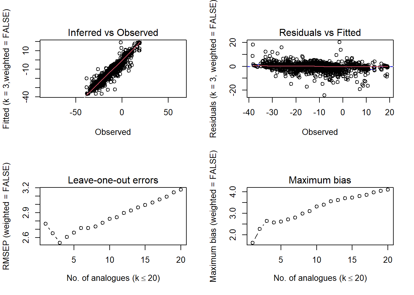
Before reconstructing environmental variables from fossil pollen assemblages, we usually assess how MAT performs in the modern species assemblage. This step is usually referred to as calibration or cross-validation.
In cross-validation, a calibration function is trained on one portion of the modern species assemblages (calibration set) and applied to another portion of the modern species assemblages (validation set). These two datasets are thus mutually exclusive and - possibly - independent. To cross-validate MAT, we usually use a technique called \(k\)-fold cross-validation. In \(k\)-fold cross-validation the modern data set is split into \(k\) mutually exclusive subsets. For each \(k^{th}\) subset, the calibration dataset comprises all the samples not in \(k\), while the samples in \(k\) comprise the validation dataset. The simplest form of \(k\)-fold cross-validation is the leave-one-out (LOO) technique, in which just a single sample is removed and then all other samples are used to build a prediction for that sample. This procedure is then repeated for all samples. The analogue package uses leave-one-out cross-validation.
Standard metrics include root mean square error (RMSE) and \(R^2\). Here, we’ll use the cross-validation tools built into the analogue package.
Note that the palaeoSig package, developed by Richard Telford, has additional functions that can test for significance relative to randomly generated variables with the same spatial structure as the environmental variable of interest. We won’t use this package in this lab, but it’s useful for testing whether apparently strong cross-validation results are merely an artifact of spatial autocorrelation (Telford and Birks 2005).
Now let’s do the analysis! First is the cross validation of the modern datasets. Using the modern data, we’ll build a calibration dataset and run cross-validation analyses of the calibration dataset. If you portaled here and skipped the Data Wrangling in Section 7.2.1, make sure you load in the pre-formatted data from Section 7.1.
    Modern Analogue Technique

Call:
mat(x = mod_pol_east_join, y = mod_jant, method = "SQchord")

Percentiles of the dissimilarities for the training set:

   1%    2%    5%   10%   20%
0.207 0.272 0.385 0.502 0.670

Inferences based on the mean of k-closest analogues:

  k  RMSEP     R2 Avg Bias Max Bias
  1  2.766  0.934   -0.214   -1.625
  2  2.654  0.939   -0.302   -2.265
  3  2.537  0.944   -0.360   -2.648
  4  2.608  0.941   -0.350   -2.569
  5  2.661  0.938   -0.357   -2.622
  6  2.714  0.936   -0.361   -2.714
  7  2.716  0.936   -0.373   -2.804
  8  2.734  0.935   -0.368   -2.982
  9  2.779  0.933   -0.357   -3.104
 10  2.826  0.930   -0.370   -3.316

Inferences based on the weighted mean of k-closest analogues:

  k RMSEP    R2 Avg Bias Max Bias
  1   NaN    NA      NaN    -1.62
  2   NaN    NA      NaN    -2.19
  3   NaN    NA      NaN    -2.52
  4   NaN    NA      NaN    -2.46
  5   NaN    NA      NaN    -2.52
  6   NaN    NA      NaN    -2.59
  7   NaN    NA      NaN    -2.68
  8   NaN    NA      NaN    -2.81
  9   NaN    NA      NaN    -2.93
 10   NaN    NA      NaN    -3.11
par(mfrow =c(2,2))plot(modpoll_jant)
Much of the information in this chapter comes from Simpson (2007), and we recommend Simpson (2007) for the interpretation of the outputs. The MAT method shares similar considerations as calculating dissimilarity (Chapter 6). With some additional considerations regarding transfer functions:
Time intervals and chronological uncertainties are not accounted for. The difference in time between successive samples often varies in palaeo-data.
Time averaging is not taken into account, and each sample may contain a different time-span of ecological productivity.
Squared chord distance is one of many distance measures available in analogue, and may not always be the most appropriate.
For deeper considerations of reconstructing temperatures using transfer functions see Telford and Birks (2005).
7.2.3 Novelty and Paleoclimatic Reconstruction
Jack action point Section needs some info from the lecture content to help understand the process as a stand-alone unit.
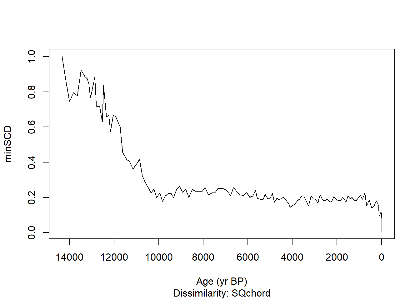
For this part of the lab, we’ll first assess the novelty of the fossil pollen assemblages at Devil’s Lake. We’ll then reconstruct past climates at Devil’s Lake, using the MAT. Here’s some demonstration code showing the kinds of analyses that can be done and plotted timeseries.
Construct a time series of the minimum SCDs (novelty) for Devil’s Lake.
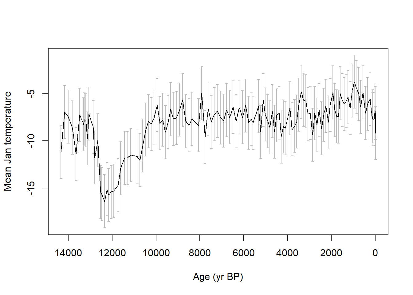
# Predict temperatures from the fossil data and their modern analoguedevil_jant <-predict(modpoll_jant, devils_prop, k=10)par(mfrow =c(1,1))devil_mindis <-minDC(devil_jant)plot(devil_mindis, depths = devils_ages, quantiles =FALSE, xlab ="Age (yr BP)", ylab ="minSCD")
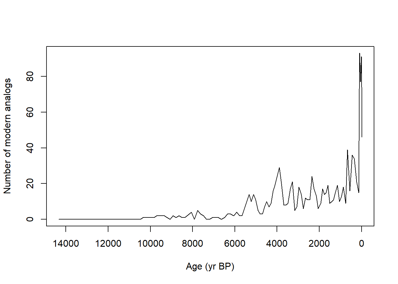
Construct a time series of the number of modern analogs found per fossil sample, using 0.25 as our no-analog/analog threshold.
devil_cma <- analogue::cma(devil_jant, cutoff=0.25)plot(x = devils_ages, y = devil_cma$n.analogs, type ="l", xlim=rev(range(devils_ages)), xlab ="Age (yr BP)", ylab ="Number of modern analogs")
Plot the reconstructed January temperatures at Devil’s Lake:
Copy in a list of DOIs for essential reading and I’ll add insert them as formatted citation links:
DOI
DOI
7.3 Part 3: Exercises
Jacktion point: review questions and question order :)
In the summary output for JanT, which choice of k (number of analogues) produces the highest R2 and lowest RMSEP?
Which samples at Devil’s Lake lack modern analogs?
Repeat the above analysis for TJul, PJul, GDD5, and MIPT. (GDD5 is growing degree days and is a measure of growing season length and strength; MIPT is an index of soil moisture availability).
Which variable has the best cross-validation statistics?
Which has the worst?
Given what you know about the climatic controls on plant distributions (and/or our ability to precisely quantify these variables), is the relative predictive skill for these different climatic variables surprising or unsurprising? Why?
Check the Devil’s Lake novelty curve against the pollen diagram for Devil’s Lake. What combinations of pollen taxa produce these no-analog assemblages?
According to Webb(1986), what are two general hypotheses for why we might have these past mixtures of species with no modern analogue?
Why should one be dubious about the temperature reconstructions at Devil’s Lake for the high-novelty assemblages?
Even for the low-novelty assemblages, name two potentially important sources of uncertainty in MAT-based reconstructions of past climate from fossil pollen data.
Conversely, based on our knowledge about the geographic climatic distributions of these taxa, why might one argue that these January temperature reconstructions are plausible?
To get practice, make reconstructions of GDD5 and mean July precipitation. Show plots of your work.
Chevalier, Manuel, Basil A. S. Davis, Oliver Heiri, Heikki Seppä, Brian M. Chase, Konrad Gajewski, Terri Lacourse, et al. 2020. “Pollen-Based Climate Reconstruction Techniques for Late Quaternary Studies.”Earth-Science Reviews 210 (November): 103384. https://doi.org/10.1016/j.earscirev.2020.103384.
Gavin, Daniel G, W.Wyatt Oswald, Eugene R Wahl, and John W Williams. 2003. “A Statistical Approach to Evaluating Distance Metrics and Analog Assignments for Pollen Records.”Quaternary Research 60 (3): 356–67. https://doi.org/10.1016/S0033-5894(03)00088-7.
Jackson, Stephen T., and John W. Williams. 2004. “Modern Analogs in Quaternary Paleoecology: Here Today, Gone Yesterday, Gone Tomorrow?”Annual Review of Earth and Planetary Sciences 32 (1): 495–537. https://doi.org/10.1146/annurev.earth.32.101802.120435.
Krause, Teresa R., James M. Russell, Rui Zhang, John W. Williams, and Stephen T. Jackson. 2019. “Late Quaternary Vegetation, Climate, and Fire History of the Southeast Atlantic Coastal Plain Based on a 30,000-Yr Multi-Proxy Record from White Pond, South Carolina, USA.”Quaternary Research 91 (2): 861–80. https://doi.org/10.1017/qua.2018.95.
Overpeck, J. T., T. Webb, and I. C. Prentice. 1985. “Quantitative Interpretation of Fossil Pollen Spectra: Dissimilarity Coefficients and the Method of Modern Analogs.”Quaternary Research 23 (1): 87–108. https://doi.org/10.1016/0033-5894(85)90074-2.
Radeloff, Volker C., John W. Williams, Brooke L. Bateman, Kevin D. Burke, Sarah K. Carter, Evan S. Childress, Kara J. Cromwell, et al. 2015. “The Rise of Novelty in Ecosystems.”Ecological Applications 25 (8): 2051–68. https://doi.org/10.1890/14-1781.1.
Simpson, Gavin L. 2007. “Analogue Methods in Palaeoecology: Using the Analogue Package.”Journal of Statistical Software 22 (September): 1–29. https://doi.org/10.18637/jss.v022.i02.
Telford, R. J., and H. J. B. Birks. 2005. “The Secret Assumption of Transfer Functions: Problems with Spatial Autocorrelation in Evaluating Model Performance.”Quaternary Science Reviews 24 (20-21): 2173–79. https://doi.org/10.1016/j.quascirev.2005.05.001.
Whitmore, J., K. Gajewski, M. Sawada, J. W. Williams, B. Shuman, P. J. Bartlein, T. Minckley, et al. 2005. “Modern Pollen Data from North America and Greenland for Multi-Scale Paleoenvironmental Applications.”Quaternary Science Reviews 24 (16-17): 1828–48. https://doi.org/10.1016/j.quascirev.2005.03.005.
Williams, J. W., and B. Shuman. 2008. “Obtaining Accurate and Precise Environmental Reconstructions from the Modern Analog Technique and North American Surface Pollen Dataset.”Quaternary Science Reviews 27 (7-8): 669–87. https://doi.org/10.1016/j.quascirev.2008.01.004.