# Load up the package
if (!require("pacman")) install.packages("pacman", repos="http://cran.r-project.org")
pacman::p_load(Bchron, splines) # splines comes with BASE-R3 Age-depth modelling
3.1 Part 1: Background
A foundational difference between geology and ecology is that, for geologists, time is an unknown variable that must be estimated with uncertainty. In contrast, most ecologists can assume that the temporal coordinates of their observations are known precisely, with zero uncertainty. Fortunately, geochronologists have a wide variety of natural clocks, thanks to the constant decay rates of radioactive isotopes. Each isotope has a unique decay rate, and so each is appropriate for particular timescales.
For the last 50,000 years, radiocarbon (14C), with its half-life of 5,730 years, is by far the most common form of radiometric dating. (Beyond 10 half-lives, so much of a radioactive substance has decayed away that it becomes immeasurable.) Radiocarbon is the mainstay of Quaternary dating and archaeology.
In Quaternary paleoecology, radiocarbon dating is expensive – a single sample typically costs $300 to $500 – so usually a given lake-sediment record will have only a scattering (ca. 5 to 30) of radiocarbon dates and other age controls. Other kinds of age controls include volcanic ash layers (tephras), 210Pb (half-life: 22.6 yrs), optically stimulated luminescence (OSL) dates, historic events such as the rise in Ambrosia pollen abundances associated with EuroAmerican land clearance, etc. An age-depth model must be constructed to estimate the age of sediments not directly associated with an age control. In multi-site data syntheses, the number of age controls, their precision, and their likely accuracy are all fundamental indicators of data quality (e.g. Blois et al. 2011; Mottl et al. 2021).
To estimate ages for depths lacking radiocarbon date, an age-depth model is required. Age-depth models are fitted to the available age controls (age estimates with uncertainty for individual depths) and provide estimates of age as a function of depth, for all depths and ages within the temporal bounds of the model.
3.2 Part 2: Code
Here we will gain practice in working with age-depth models of various kind, and assessing their age estimates and uncertainty. We’ll begin with a bit of practice in calibrating radiocarbon years to calendar years and comparing the resulting age estimates from different calibration curves.
Packages required for this section
We will be using Bchron for calibration and Bayesian age-depth modelling. Notably rbacon is another commonly used package, see Trachsel and Telford (2017) for a discussion on age-depth models. We will also be fitting some interpolation and linear models using BASE-R. Remember you must have packages both installed and loaded, often loading a package is done via the library(packagename) function. The following code using the pacman package takes care of installation and loading in one go.
3.2.1 Calibration of Radiocarbon Dates
A complication in radiocarbon dating is that the initial calculation of a radiocarbon age assumes, by convention, that the amount of radiocarbon in the atmosphere is constant over time. See Bronk Ramsey (2008) for a good overview of 14C dating. This assumption is untrue, so all radiocarbon age estimates must be post-hoc calibrated using a calibration curve that is based on compiling radiocarbon dates of materials that have precise independent age estimates (e.g. tree rings, corals). The IntCal series (IntCal04, IntCal09, IntCal13, IntCal20) is the community standard for calibrating radiocarbon dates to age estimates in calendar years (e.g., Reimer et al. 2020). The conversion from radiocarbon to calendar years usually further increases the uncertainty of age estimates.
Yet another complication in radiocarbon dating is that different calibration curves need to be used for the Northern vs. Southern Hemisphere and for the atmosphere vs. oceans, due to different residence times of 14C in these different reservoirs. For example, atmospheric radiocarbon that diffuses into the surface oceans usually will reside for centuries before phytoplankton biologically fix it through photosynthesis, which will lead marine 14C to be depleted (and ‘too old’) relative to atmospheric 14C. Use the wrong calibration curve and your age estimate will be inaccurate!
3.2.1.1 Calibrating radiocarbon dates in R
Here we’ll experiment with calibrating radiocarbon dates, using various calibration curves. Radiocarbon dated samples come back from the lab with a radiocarbon age and standard deviation, among other information. These two bits of information are used to calibrate the radiocarbon dates to estimated ages. R packages may have useful vignettes (package tutorials) and built-in datasets that provide handy test templates. The following code is modified from the Bchron vignette.
ages = BchronCalibrate(ages=c(3445,11553,7456),
                        ageSds=c(50,230,110),
calCurves=c('intcal20','intcal20','intcal20'))summary(ages)95% Highest density regions for Date1
$`94.4%`
[1] 3572 3834
95% Highest density regions for Date2
$`0.4%`
[1] 13004 13025
$`77.9%`
[1] 13059 13874
$`16.4%`
[1] 13923 14012
95% Highest density regions for Date3
$`94.6%`
[1] 8022 8423plot(ages)[[1]]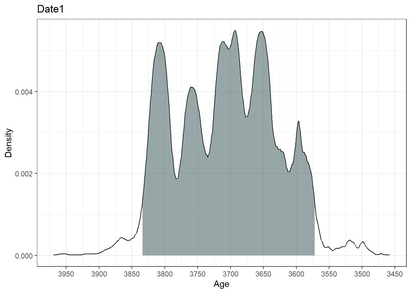
[[2]]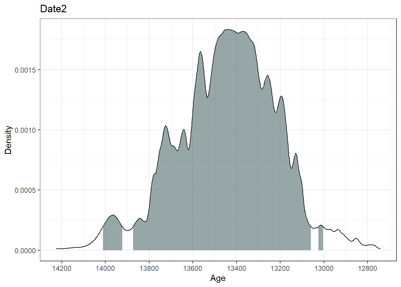
[[3]]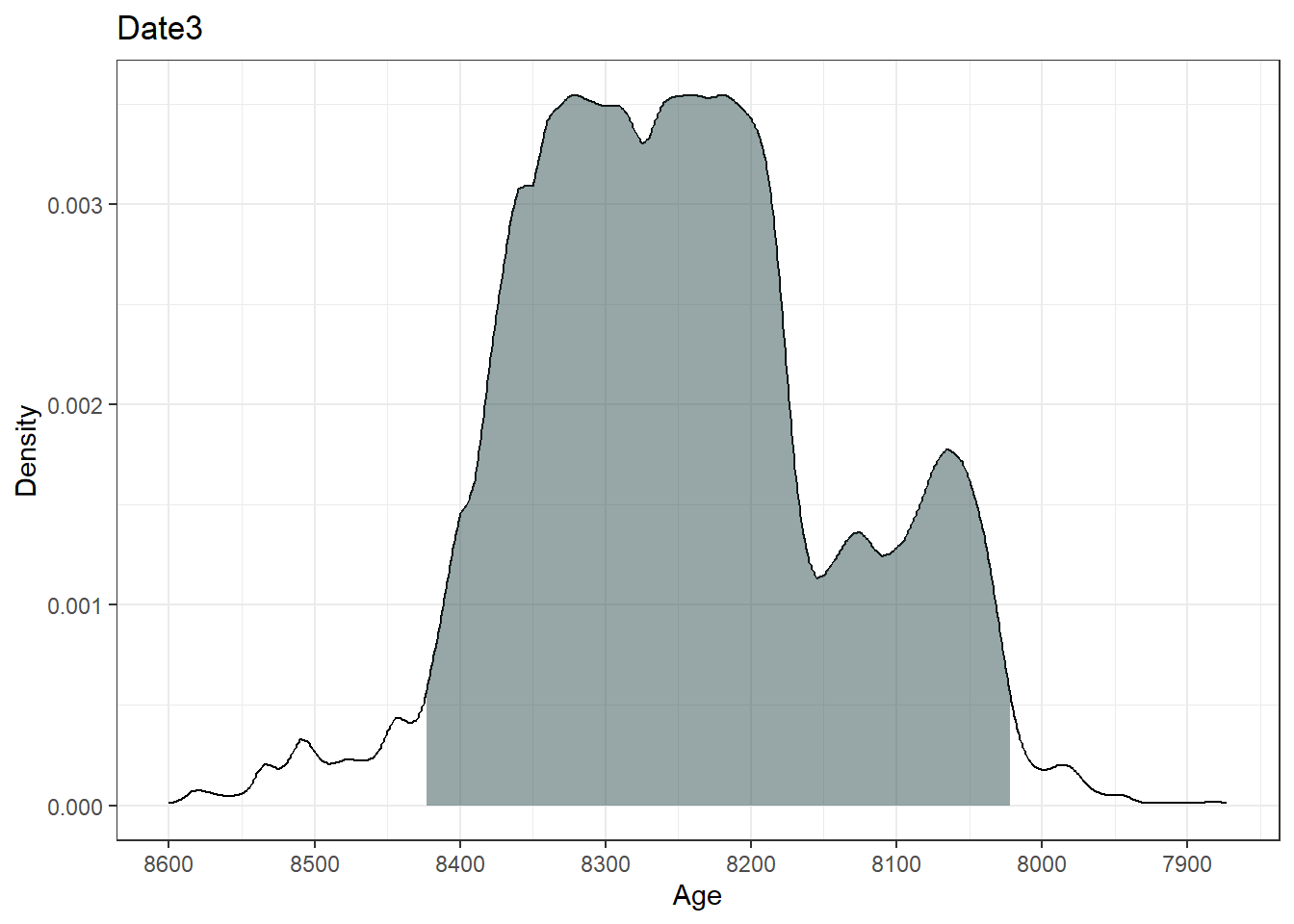
plot(ages, includeCal = TRUE, fillCol = 'red')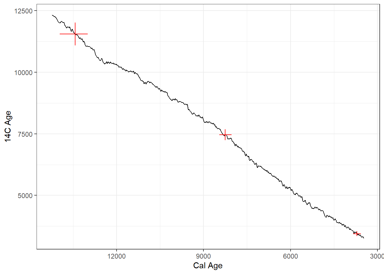
The output summary indicates the range of the highest density regions (i.e., the most likely ‘real’ age range of the sample). The plot function in Bchron outputs a ggplot object of the high density regions of the most likely ages.
3.2.2 Types of Age-Depth Models
Different kinds of age-depth models exist, each with their own underlying assumptions and behavior. In the list below, #1-4 are classical or traditional forms of age-depth models, but Bayesian models are now the norm. The packages rbacon (usually referred to as ‘bacon’) and Bchron are the current standards for Bayesian age-depth modelling. Before going to bayesian models, we’ll begin with the classics.
Linear interpolation, a.k.a. ‘connect the dots,’ in which straight lines are drawn between each depth-adjacent pair of age controls.
Linear regression (\(y=b0~ + b1x\); \(y=\)time and \(x=\)depth; \(b0\) and \(b1\) are constants), in which a single straight line is fitted through the entire set of age controls. In ordinary linear regression (OLS), the chosen line will minimize the y-dimension distances of individual points to the line. Standard OLS assumes that all observations are normally distributed, which is a poor assumption for calibrated radiocarbon dates.
Polynomials, also fitted to the entire set of age controls (\(y= b0 + b1x + b2x^2 + b3x^3 + …bnx^n\)), are an extension of linear regression, with additional terms for \(x^2\), \(x^3\), etc. Some arbitrary maximum n is chosen, usually in the range of 3 to 5. These are called ‘third-order polynomials,’ ‘fifth-order polynomials,’ etc.
Splines, which are a special kind of polynomial function that are locally fitted to subsets of the age controls, and then smoothly interpolated between points. (Several different formulas can be used to generate splines; common forms include cubic, smooth, monotonic, and LOWESS).
Bayesian age models (e.g.
bacon,bchron,oxcal, etc.). Bayesian models differ in detail, but all combine a statistical representation of prior knowledge with the new data (i.e. the age controls at a site) to build an age-depth model with posterior estimates of age for any given depth. Bayesian models are now widely used because- they allow the incorporation of prior knowledge (e.g., from coring many lakes, we now have decent estimates of typical sediment accumulation rates, Goring et al. (2012));
- they can handle highly irregular probability distribution functions such as those for radiocarbon dates after calibration; and as a result
- they generally do a better job of describing uncertainty than traditional age-depth models.
3.2.2.1 Classical age-depth models
Classical models are now out-dated methods (Blaauw et al. 2018), but it is useful to understand how they work as literature before the relatively recent development of Bayesian methods has relied on them. Let’s explore some classical methods of age-depth modelling using one of the datasets included with the Bchron package. The data are from a core in Northern Ireland; Sluggan Bog Smith and Goddard (1991), and can be called via:
data(Sluggan) # Call the data from Bchron
print(Sluggan) # Check out the data
Linear interpolation predicts ages by simply, drawing a line between successive dated samples. This method assumes that there is a constant age-depth relationship between samples. An assumption that is unlikely to be true, especially of cores with fewer dated samples than Sluggan Moss.
interp_ages <- approx(x = Sluggan$ages, y = Sluggan$position) # use the function approx() to interpolate between ages
plot(x = interp_ages$x, y = interp_ages$y, type = 'l') # Plot the interpolated data
points(x = Sluggan$ages, y = Sluggan$position, cex = 1.5, col = 'red') # overlay the original age points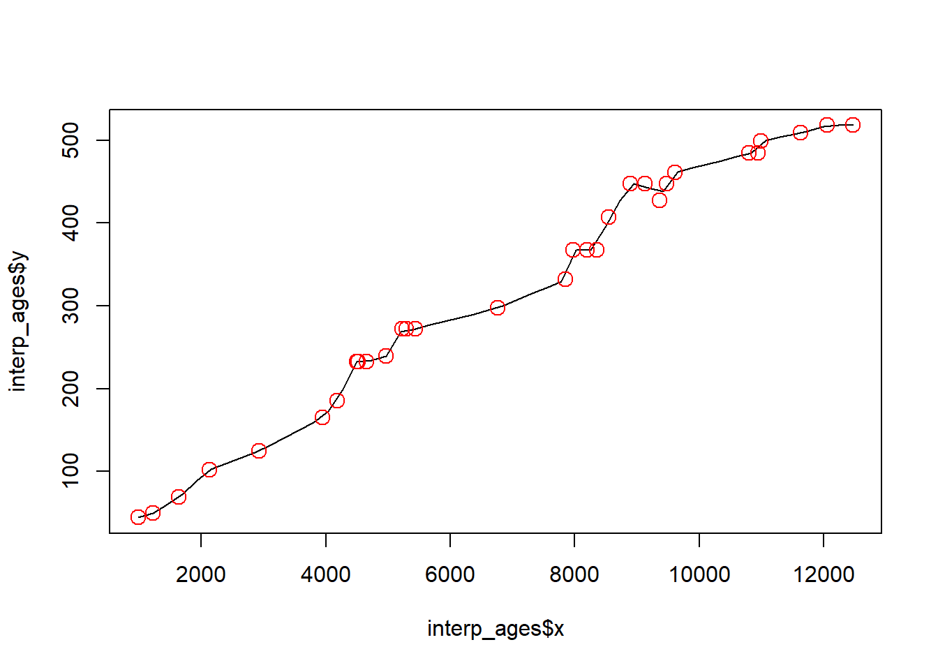
Linear regression provides a line of best fit through the dated samples. This method assumes a constant age-depth relationship across all samples, also unlikely to be true depending on processes affecting the core during its formation.
mod_ages <- lm(Sluggan$position ~ Sluggan$ages) # Create a linear regression model
plot(x = Sluggan$ages, y = Sluggan$position, cex = 1.5, col = 'red') # Plot the original ages
abline(mod_ages) # add the regression line from the regression model
Polynomial regression allows a curve to be fit through the data. The amount the curve ‘wiggles’ depends on the order of the polynomial fit to the data. Polynomial regression has the risk of being over-fit.
x <- Sluggan$ages # Renaming the variables because the predict function below is fussy about the input name
y <- Sluggan$position
poly_ages <- lm(y ~ poly(x, 3))

plot(x = Sluggan$ages, y = Sluggan$position, cex = 1.5, col = 'red')
age_range <- seq(from = range(Sluggan$ages)[1], to = range(Sluggan$ages)[2], length.out = 250)
lines(age_range, predict(poly_ages, data.frame(x = age_range)))
Splines are a class of functions including, for example, smoothing splines or cubic splines. Cubic splines are pieve-wise polynomials locally between ‘knots’. That is the data are split into bins that are fit independently using. By default, the bs() function uses a third degree polynomial. Without providing knots the fit will look the same as a third degree polynomial regression.
cubic_ages <- lm(y ~ bs(x, knots = c(1000, 6000, 12000)))
plot(x = Sluggan$ages, y = Sluggan$position, cex = 1.5, col = 'red')
lines(age_range, predict(cubic_ages, data.frame(x = age_range)))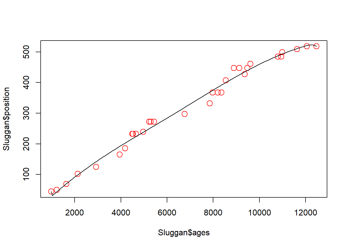
Because classical age-depth modelling is rarely used now we are not going to delve further into the statistical details of the best way of fitting each model (e.g., the number of knots to use for fitting a cubic spline).
One of the issues with classical age-depth modelling is that uncertainty decreases with fewer datapoints.
3.2.2.2 Bayesian age-depth models
Now let’s see what the latest methods show for the same dataset.
Note that all the values provided to the arguments are contained in the Sluggan dataframe. When creating chronologies from your own (or accessed data), you may need to rename them to match your data.
SlugganOut = with(Sluggan,
               Bchronology(ages=ages,
                           ageSds=ageSds,
                           calCurves=calCurves,
                           positions=position,
                           positionThicknesses=thickness,
                           ids=id,
                           predictPositions=seq(0,518, by=10)))
The summary shows for each position (depth) the median and quartiles of the predicted ages for that position.
summary(SlugganOut)Quantiles of predicted ages by depth:
Depth 2.5% 25% 50% 75% 97.5%
0 -52.025 118.75 280.5 453.00 747.075
10 57.975 269.00 430.5 564.25 790.050
20 164.950 420.75 553.5 675.00 837.025
30 283.975 557.00 668.0 765.25 883.075
40 521.950 727.75 796.5 853.00 927.000
50 959.975 1065.00 1130.5 1193.00 1331.150
60 1142.000 1275.00 1336.0 1397.00 1546.050
70 1402.000 1488.75 1549.0 1622.25 1778.050
80 1513.000 1651.00 1740.5 1833.00 2059.050
90 1621.900 1811.75 1901.0 2004.00 2173.025
100 1842.950 2006.00 2078.0 2162.25 2278.000
110 2173.925 2369.00 2473.0 2600.25 2913.050
120 2397.975 2724.75 2845.5 2946.00 3116.025
130 2964.000 3154.75 3275.0 3430.25 3809.000
140 3099.875 3390.00 3566.5 3764.25 4073.000
150 3268.850 3637.75 3845.5 4016.25 4250.050
160 3570.925 3968.00 4124.5 4224.25 4395.050
170 4205.975 4342.00 4423.0 4497.25 4640.050
180 4344.875 4499.00 4572.0 4643.00 4779.000
190 4528.000 4666.75 4741.5 4813.00 4943.000
200 4605.925 4746.00 4832.0 4906.00 5047.125
210 4657.950 4827.75 4910.0 4985.25 5117.175
220 4753.925 4909.00 4986.0 5056.25 5195.000
230 4870.000 5022.00 5085.5 5146.00 5266.100
240 5534.975 5634.00 5674.0 5725.00 5850.000
250 5638.950 5736.75 5788.0 5849.00 5962.125
260 5718.975 5829.75 5886.0 5934.25 6036.025
270 5846.975 5939.00 5989.0 6029.25 6124.025
280 6300.975 6484.00 6621.0 6832.50 7267.250
290 6536.975 6975.00 7171.0 7315.25 7535.025
300 7498.950 7622.00 7691.0 7788.00 8103.100
310 7641.000 7828.00 7950.0 8129.25 8424.100
320 7782.950 8061.75 8229.0 8356.25 8590.025
330 8119.900 8397.00 8478.0 8583.00 8773.025
340 8477.000 8606.75 8692.0 8777.00 8953.050
350 8547.925 8697.75 8791.0 8886.25 9038.125
360 8627.850 8796.75 8890.0 8983.25 9119.075
370 9074.975 9232.00 9302.0 9389.00 9522.025
380 9147.950 9322.00 9408.5 9481.00 9687.025
390 9236.850 9400.00 9476.0 9566.50 9791.025
400 9317.925 9473.00 9556.5 9655.25 9903.625
410 9510.975 9643.00 9752.0 9866.00 10142.150
420 9621.975 9858.75 9982.5 10105.25 10274.000
430 9843.750 10065.75 10261.5 10323.00 10456.075
440 9953.975 10172.00 10310.0 10383.25 10532.075
450 10442.000 10596.00 10692.0 10804.25 11040.050
460 10713.000 10923.75 11017.5 11107.00 11283.000
470 11153.000 11522.00 11731.0 11931.25 12445.200
480 11547.950 12236.75 12411.5 12546.25 12720.025
490 12748.975 12864.00 12924.5 12984.00 13104.050
500 12910.000 13050.00 13113.0 13180.00 13369.050
510 13315.925 13490.75 13585.5 13686.00 13925.025plot(SlugganOut)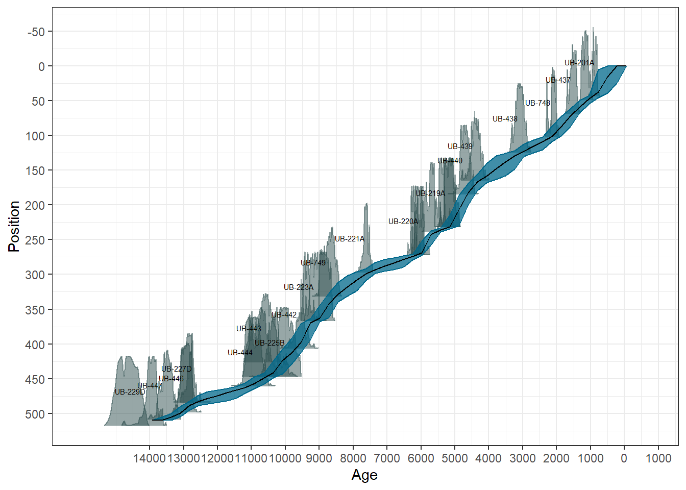
A more complete version of the modelling process using Bchron can be found in the vignette.
Resources
Age-depth modelling is complicated, there are many pitfalls, assumptions, and uncertainties that are often ignored. Recent developments have begun to focus on quantifying uncertainties to understand the reliability of inferences made from the data. Key papers for understanding age depth modelling include:
3.3 Part 3: Exercises
You may want to refer to the bchron vignette to find some helpful information for the exercises below.
3.3.1 Calibration
- Using the existing example code, change the
calCurvesinput to:- the Southern Hemisphere calibration curve
- the marine sediments curve.
- Calibrate a different set of three ages by modifying the inputs to
agesandageSds.
The object you assigned the result of BchronCalibrate to contains all the calibration information and can be accessed with the $ e.g., ages$Date1$ageGrid
- Using one of your calibrated sets of three dates, calculate the median age from the
ageGridand the difference of each calibrated age to the original uncalibrated age.
Median and mean ages
Commonly, only the median age is reported; however, it is good practice to report and consider the range of possible ages, especially when exploring synchroneity of events across space. Notice how Bchron focuses on delivering ranges and densities.
3.3.2 Classical age-depth modelling:
Bchronhas a second built-in dataset named Glendalough. Using the Glendalough dataset:- Fit a linear interpolation, linear regression, three different order polynomials and a cubic spline
- Plot the results
- Did you run into any errors or warnings? If so, why?
3.3.3 Bayesian age-depth modelling
- Run the
Bchronage-depth model on the Glendalough dataset and consider:- How does uncertainty change between the plot outputs between the Glendalough (a dataset with fewer radiocarbon dates) and Sluggan Moss (a data-rich site)
- Run the summary funcion on the Glendalough model, does the output reflect the plot? Is there smaller uncertainty around samples? Why is interpreting results in the context of the uncertainty important?