# Load up the package
if (!require("pacman")) install.packages("pacman", repos="http://cran.r-project.org")
pacman::p_load(dplyr, ggplot2, neotoma2, sf, geojsonsf, leaflet, raster, DT, rioja, htmlwidgets) # Pacman will load neotoma24 The neotoma2 package
4.1 Part 1: Background
This series of exercises is designed to give you hands-on practice in using the neotoma2 R package (Goring et al. 2015), both for practical reasons and for insights into how open-data systems work. This section is a condensed version of the current workshop and focuses on data structures and the core functions in the neotoma2 R package for downloading and manipulating data. A hard-won lesson for a practicing data scientist is how much time and attention goes into data handling! For a more extended introduction to Neotoma, see the current workshop. If you’re planning on working with Neotoma more in the future, please join us on Slack, where we manage a channel specifically for questions about the R package. You may also wish to join Neotoma’s Google Groups mailing list, and if so contact us to be added.
This series of exercises is designed to give you hands-on practice in using APIs and the neotoma2 R package, both for practical reasons and for insights into how open-data systems work. neotoma2’s primary purpose is to pass data from the Neotoma DB server into your local R computing environment.
In this tutorial you will learn how to:
Search for sites using site names and geographic parameters
Filter results using temporal and spatial parameters
Obtain sample information for the selected datasets
4.2 Part 2: Getting Started With neotoma2
The primary purpose of neotoma2 is to pass data from the Neotoma Paleoecology Database (Neotoma DB) server into your local R environment. neotoma2 has a layered structure of core functions for obtaining data:
- sites
- datasets
- downloads
- samples
There are many more functions for maipulating data and conducting other operations that we will encounter along the way while we take you through these four data layers. For this workbook we use several packages, including leaflet, sf and others. We load the packages using the pacman package, which will automatically install the packages if they do not currently exist in your set of packages.
Packages required for this section
4.2.1 Good coding practice: explicitly naming packages and functions
Different packages in R are created independently by different teams of developers, and it’s very common for two different packages to use the same function names. This can lead to coding errors if you call a function that you know is in one package, but R guesses wrongly that you wanted a function of the same name from an entirely different package. For example, for a function like filter(), which exists in both neotoma2 and other packages such as dplyr, you may see an error that looks like:
Oh no! 😱
Error in UseMethod("filter") :
 no applicable method for 'filter' applied to an object of class "sites"
You can avoid this error by explicitly naming which package has the function that you want to use, through the standard convention of double colons (package.name::function.name). For example, using neotoma2::filter() tells R explicitly that you want to use the filter() function in the neotoma2 package, not some other package version.
4.3 Neotoma2: Site Searches: get_sites()
Many users of Neotoma first want to search and explore data at the site level. There are several ways to find sites in neotoma2, but we think of sites primarily as spatial objects. They have names, locations, and are found within geopolitical units. However, sites themselves do not have associated information about taxa, dataset types, or ages. sites instead are simply the container into which we add that information. So, when we search for sites we can search by:
- siteid
- sitename
- location
- altitude (maximum and minimum)
- geopolitical unit
4.3.0.1 Searching by Site Name: sitename="%Devil%"
We may know exactly what site we’re looking for (“Devil’s Lake”), or have an approximate guess for the site name (for example, we know it’s something like “Devil Pond”, or “Devil’s Hole”).
We use the general format: get_sites(sitename="XXXXX") for searching by name.
PostgreSQL (and the API) uses the percent sign as a wildcard. So "%Devil%" would pick up “Devils Lake” for us (and would pick up “Devil’s Canopy Cave”). Note that the search query is case insensitive, so "%devil%" will work.
If we want an individual record we can use the siteid, which is a unique identifier for each site: .
devil_sites <- neotoma2::get_sites(sitename = "%Devil%")
plotLeaflet(devil_sites)
4.3.0.2 Searching by Location: loc=c()
The neotoma package used a bounding box for locations, structured as a vector of latitude and longitude values: c(xmin, ymin, xmax, ymax). The neotoma2 R package supports both this simple bounding box and also more complex spatial objects, using the sf package. Using the sf package allows us to more easily work with raster and polygon data in R, and to select sites using more complex spatial objects. The loc parameter works with the simple vector, WKT, geoJSON objects and native sf objects in R. Note however that the neotoma2 package is a wrapper for a simple API call using a URL (see APIs above), and URL strings have a maximum limit of 1028 characters, so the API currently cannot accept very long/complex spatial objects.
As an example of different ways that you can search by location, let’s say you wanted to search for all sites in the state of Michigan. Here are three spatial representations of Michigan: 1) a geoJSON list with five elements, 2) WKT, and 3) bounding box representation. And, as a fourth variant, we’ve transformed the mich$geoJSON element to an object for the sf package. Any of these four spatial representations work with the neotoma2 package.
mich <- list(geoJSON = '{"type": "Polygon",
        "coordinates": [[
            [-86.95, 41.55],
            [-82.43, 41.55],
            [-82.43, 45.88],
            [-86.95, 45.88],
            [-86.95, 41.55]
            ]]}',
        WKT = 'POLYGON ((-86.95 41.55,
                         -82.43 41.55,
                         -82.43 45.88,
                         -86.95 45.88,
                         -86.95 41.55))',
        bbox = c(-86.95, 41.55, -82.43, 45.88))

mich$sf <- geojsonsf::geojson_sf(mich$geoJSON)[[1]]

mich_sites <- neotoma2::get_sites(loc = mich$geoJSON, all_data = TRUE)
You can always simply plot() the sites objects, but this won’t show any geographic context. The leaflet::plotLeaflet() function returns a leaflet() map, and allows you to further customize it, or add additional spatial data (like our original bounding polygon, mich$sf, which works directly with the R leaflet package):
neotoma2::plotLeaflet(mich_sites) %>%
  leaflet::addPolygons(map = .,
                       data = mich$sf,
                       color = "green")
4.3.0.3 Helper Functions for Site Searches

If we look at the UML diagram for the objects in the neotoma2 R package, we can see that there are a set of functions that can operate on sites. As we add to sites objects, using get_datasets() or get_downloads(), we are able to use more of these helper functions. We can use functions like summary() to get a more complete sense of the types of data in this set of sites.
The following code gives the summary table. We do some R magic here to change the way the data is displayed (turning it into a datatable() object using the DT package), but the main function is the summary() call.
neotoma2::summary(mich_sites)We can see that there are no chronologies associated with the site objects. This is because, at present, we have not pulled in the dataset information we need. All we know from get_sites() are the kinds of datasets we have.
4.3.1 Searching for Datasets
Now that we know how to search for sites, we can start to search for datasets. As we’ve discussed before, in the Neotoma data model, each site can contain one or more collection units, each of which can contain one or more datasets. Similarly, a sites object contains collectionunits which contain datasets. From the table above, we can see that some of the sites we’ve looked at contain pollen data. However, so far we have only downloaded the sites data object and not any of the actual pollen data, it’s just that (for convenience) the sites API returns some information about datasets, to make it easier to navigate the records.
With a sites object we can directly call get_datasets(), to pull in more metadata about the datasets. At any time we can use datasets() to get more information about any datasets that a sites object may contain. Compare the output of datasets(mich_sites) to the output of a similar call using the following:
mich_datasets <- neotoma2::get_datasets(mich_sites, all_data = TRUE)

datasets(mich_datasets)
Warning in get_datasets.sites(mich_sites, all_data = TRUE): SiteID 23324, 24000, 24001, 24002, 24003, 24004, 24005, 24006, 24007, 24008, 27284, 27285, 27286, 27287, 27288, 27289, 27317, 27346, 27505, 27506 or DatasetID NA, NA, NA, NA, NA, NA, NA, NA, NA, NA, NA, NA, NA, NA, NA, NA, NA, NA, NA, NA does not exist in the Neotoma DB yet or it has been removed.
It will be removed from your search.4.3.2 Filter Records
If we choose to pull in information about only a single dataset type, or if there is additional filtering we want to do before we download the data, we can use the filter() function. For example, if we only want pollen records, and want records with known chronologies, we can filter:
mich_pollen <- mich_datasets %>%
  neotoma2::filter(datasettype == "pollen" & !is.na(age_range_young))

neotoma2::summary(mich_pollen)
Note, that we are filtering on two conditions. (You may want to look up the operators being used in the above code: ==, &, and ! to understand what they accomplish in the code.) We can see now that the data table looks different, and there are fewer total sites.
4.3.3 Retrieving sample() data.
The sample data are the actual data that scientists usually want - counts of pollen grains, lists of vertebrate fossil occurrences, etc. Because sample data can have fairly large data volumes (each dataset may contain many samples), which can strain server bandwidth and local computing memory, we try to call get_downloads() after we’ve done our preliminary filtering. After get_datasets(), you have enough information to filter based on location, time bounds, and dataset type. When we move to get_downloads() we can do more fine-tuned filtering at the analysis unit or taxon level.
The following command may take a few moments to run. (If it takes too long, we have stored an already-downloaded version of the function output as an RDS data file that you can load directly into R.)
mich_dl <- mich_pollen %>% get_downloads(all_data = TRUE)............................# mich_dl <- readRDS('data/mich_dl.rds')Once we’ve downloaded the sample data, we now have information for each site about all the associated collection units, the datasets, and, for each dataset, all the samples associated with the datasets. To extract all the samples we can call:
allSamp <- samples(mich_dl)When we’ve done this, we get a data.frame that is 40084 rows long and 37 columns wide. The reason the table is so wide is that we are returning data in a long format. Each row contains all the information you should need to properly interpret it:
 [1] "age"             "agetype"         "ageolder"        "ageyounger"
 [5] "chronologyid"    "chronologyname"  "units"           "value"
 [9] "context"         "element"         "taxonid"         "symmetry"
[13] "taxongroup"      "elementtype"     "variablename"    "ecologicalgroup"
[17] "analysisunitid"  "sampleanalyst"   "sampleid"        "depth"
[21] "thickness"       "samplename"      "datasetid"       "database"
[25] "datasettype"     "age_range_old"   "age_range_young" "datasetnotes"
[29] "siteid"          "sitename"        "lat"             "long"
[33] "area"            "sitenotes"       "description"     "elev"
[37] "collunitid"
For some dataset types, or analyses some of these columns may not be needed, however, for other dataset types they may be critically important. To allow the neotoma2 package to be as useful as possible for the community we’ve included as many as we can.
4.3.3.1 Extracting Taxa
If you want to know what taxa we have in a dataset, you can use the helper function taxa() on the sites object. The taxa() function gives us, not only the unique taxa, but two additional columns, sites and samples, that tell us how many sites the taxa appear in, and how many samples the taxa appear in, to help us better understand how common individual taxa are.
neotomatx <- neotoma2::taxa(mich_dl)The taxonid values can be linked to the taxonid column in the samples(). This allows us to build taxon harmonization tables if we choose to. Note also that the taxonname is in the field variablename. Individual sample counts are reported in Neotoma as variables. A “variable” may be either a species for which we have presence or count data, a geochemical measurement, or any other proxy, such as charcoal counts. Each stored entry for a variable includes the units of measurement and the value.
4.3.3.2 Taxonomic Harmonization (Simple)
A standard challenge in Neotoma (and in biodiversity research more generally) is that different scientists use different names for taxonomic entities such as species. Even if everyone agrees on a common taxonomy, it’s quite possible that a given fossil might be only partially identifiable, perhaps just to genus or even family. Hence, when working with data from Neotoma, a common intermediary step is to ‘harmonize’ all the taxa names stored in Neotoma into some standard names of interest to you.
Let’s say we want to know the past distribution of Pinus. We want all the various pollen morphotypes that are associated with Pinus (e.g. Pinus strobus, Pinus strobus-type, Pinus undif., Pinus banksiana/resinosa) to be grouped together into one aggregated taxon names called Pinus. There are several ways of doing this, either directly by exporting the file and editing each individual cell, or by creating an external “harmonization” table.
Programmatically, we can harmonize all the taxon names using matching and transformation. We’re using dplyr type coding here to mutate() the column variablename so that any time we detect (str_detect()) a variablename that starts with Pinus (the .* represents a wildcard for any character [.], zero or more times [*]) we replace() it with the character string "Pinus". Note that this changes Pinus in the allSamp object, but if we were to call samples() again, the taxonomy would return to its original form.
As a first step, we’re going to filter the ecological groups to include only UPHE (upleand/heath) and TRSH (trees and shrubs). (More information about ecological groups is available from the Neotoma Online Manual.) After converting all _Pinus._ records to Pinus* we then sum the counts of the Pinus records.
allSamp <- allSamp %>%
  dplyr::filter(ecologicalgroup %in% c("UPHE", "TRSH")) %>%
  mutate(variablename = replace(variablename,
                                stringr::str_detect(variablename, "Pinus.*"),
                                "Pinus"),
         variablename = replace(variablename,
                                stringr::str_detect(variablename, "Ambrosia.*"),
                                "Ambrosia")) %>%
  group_by(siteid, sitename,
           sampleid, variablename, units, age,
           agetype, depth, datasetid,
           long, lat) %>%
  summarise(value = sum(value), .groups='keep')
There were originally 6 different taxa identified as being within the genus Pinus (including Pinus, Pinus subg. Pinus, and Pinus undiff.). The above code reduces them all to a single taxonomic group Pinus. We can check out the unique names by using:
neotomatx %>%
  ungroup() %>%
  dplyr::filter(stringr::str_detect(variablename, "Pinus")) %>%
  reframe(pinus_spp = unique(variablename))

# I actually like Base here for the one-liner:
# unique(grep("Pinus", neotomatx$variablename, value = TRUE))
If we want to store a record of our choices outside of R, we can use an external table. For example, a table of pairs (what we want changed, and the name we want it replaced with) can be generated, and it can include regular expressions (if we choose):
| original | replacement |
|---|---|
| Abies.* | Abies |
| Vaccinium.* | Ericaceae |
| Typha.* | Aquatic |
| Nymphaea | Aquatic |
| … | … |
We can get the list of original names directly from the taxa() call, applied to a sites object, and then export it using write.csv(). We can also do some exploratory plots of the data:
taxaplots <- taxa(mich_dl)
# Save the taxon list to file so we can edit it subsequently.
readr::write_csv(taxaplots, "data/mytaxontable.csv")
`geom_smooth()` using formula = 'y ~ x'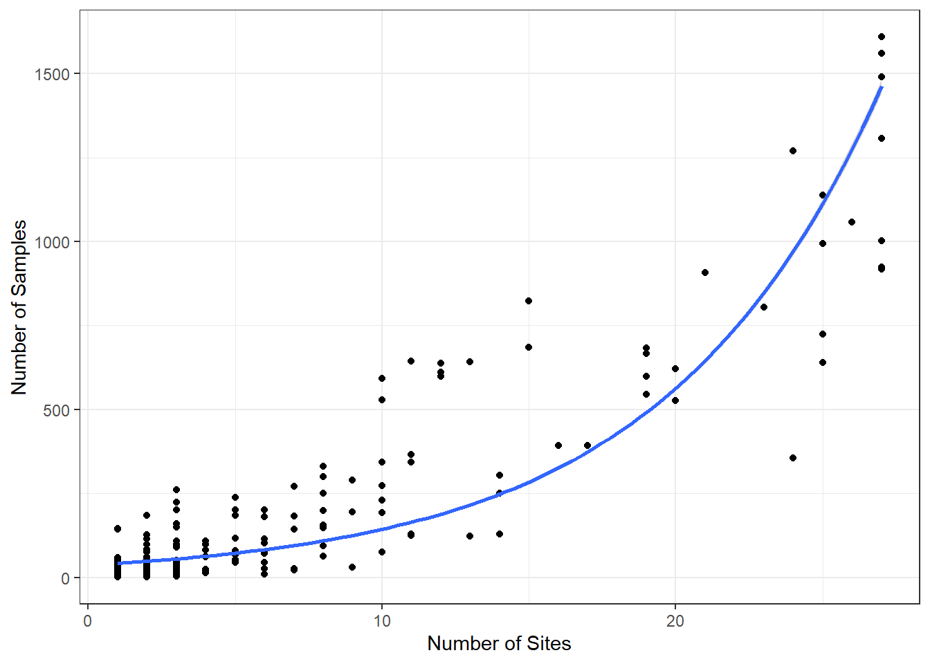
The plot is mostly for illustration, but we can see, as a sanity check, that the relationship is as we’d expect.
4.4 Conclusion
So, we’ve done a lot in this exercise. We’ve (1) learned how APIs work (2) searched for sites using site names and geographic parameters, (3) filtered results using temporal and spatial parameters, (4) built a pollen diagram, and (5) done a first-pass spatial mapping of taxa. We will build upon this methodological foundation in future lab exercises.
4.5 Part 3 Exercises
How many sites have the name ‘clear’ in them? Show both your code and provide the total count.
Which state has more sites in Neotoma, Minnesota or Wisconsin? How many in each state? Provide both code and answer.
How many different kinds of datasets are available at Devil’s Lake, WI? Show both code and answer. Ensure that your code just retrieves datasets for just this single site.
Follow the Pinus example above, but now for Picea. How many taxon names were aggregated into your Picea name?
Make a stratigraphic pollen diagram in
rioja, for a site of your choice (not Devils Lake) and taxa of your choice. Show code and resulting diagram.