Information loss in palaeoecological data
This is a sneak preview into work that is in review. A link to the published version will be added here once it is available.
In my previous post, I described the phenomenological model used to generate species patterns that mimic the statistical properties of empirical data. How can we use this approach to quantify the relative influence of sources of uncertainty on the statistical inferences we make from palaeoecological data?
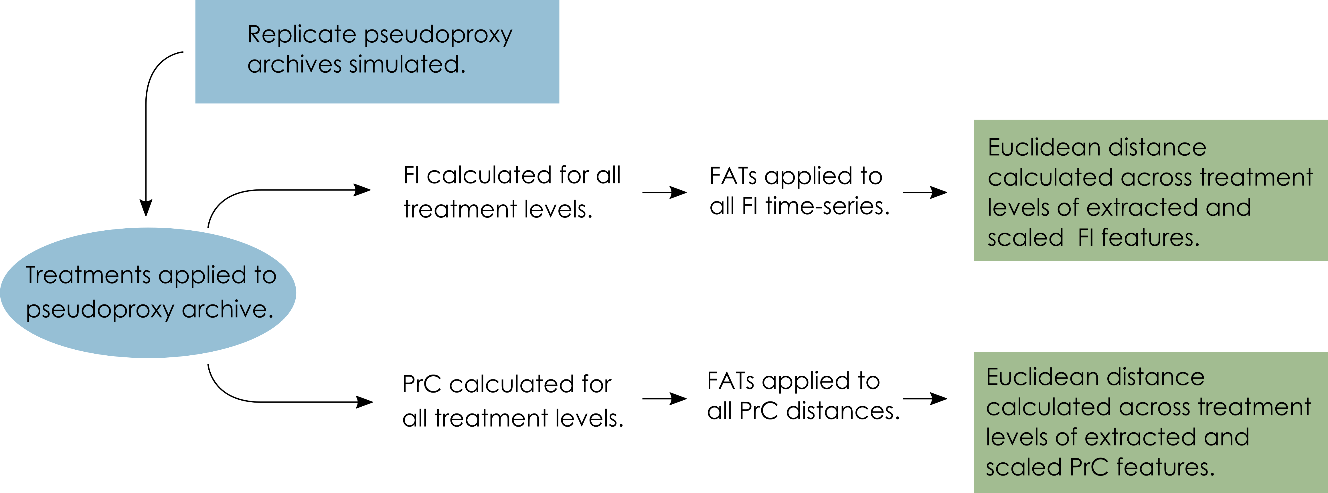
I’ll pick up where I left off in the last post. In short, we simulate a whole bunch of species and begin to systematically degrade the data with physical processes (in this case core mixing), sub-sampling strategies (taking 1 cm thick slices of sediment at given intervals), and proxy counting (counting and identifying species in a sub-sample). Because each of these three sources of uncertainty are introduced to the data individually, and combined, at 10 levels each, we end up with 1210 datasets per replicate simulation! There are 30-35 replicate simulations, multiplied by four different scenarios varying the driving conditions. That is terabytes of data! We want to know the relative influence of the three sources of uncertainty (mixing, sub-sampling, and proxy counting) on the two statistical analyses (Fisher Information and principal curves), from the ‘error-free’ benchmark to the most degraded and least intensively sampled.
To compare the Fisher Information and principal curve analyses of the ecological communities across the 1210 datasets we used Feature Analysis for Time series. This further reduces the time-series into a set of ‘features’ that describe the time-series. We can then use Euclidean distance to measure the distance between the features of each dataset and the original benchmark. These distances are then summarised across the replicate simulations (Figure 1).
Ok, the methods are not very easy to describe in simple terms… They will be described in detail when the paper comes out. So for the time being, let’s jump to the exciting results!

The uncertainties are introduced to the data systematically. By introducing the uncertainties individually, we can see how the Euclidean distance increases from our benchmark data (Figure 2). It is interesting the Euclidean distance increases steadily with mixing, while the Euclidean distance does not increase a great deal as the proxy count is reduced. Decreasing sub-sampling intervals are having the strongest influence on the Euclidean distance.
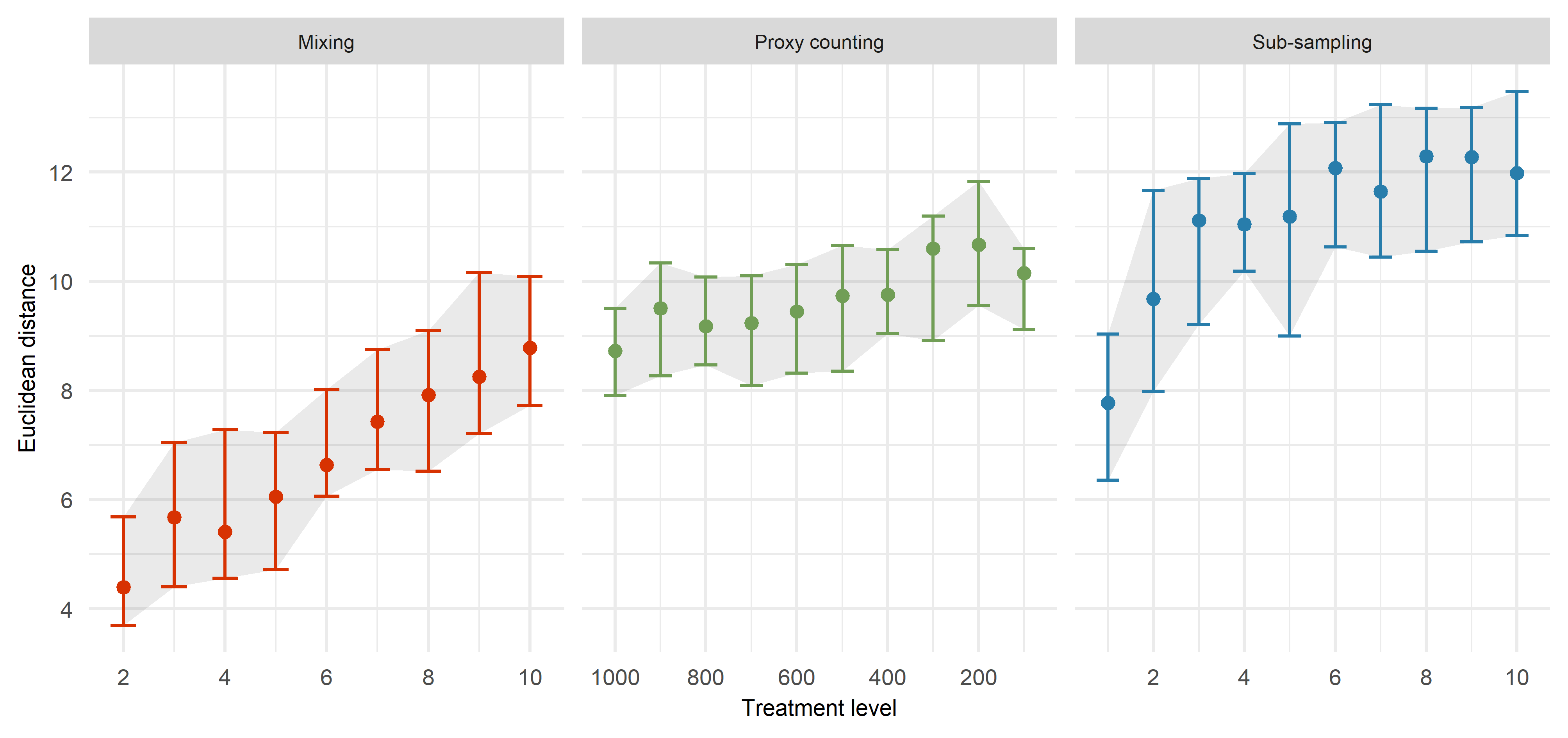
It is useful to see the different influence of the uncertainties when applied individually. However, this result is expected. We know that data become worse if we ruin them! What we want to find out is which sources of uncertainty have the strongest influence, and which ones interact when applied in combination.
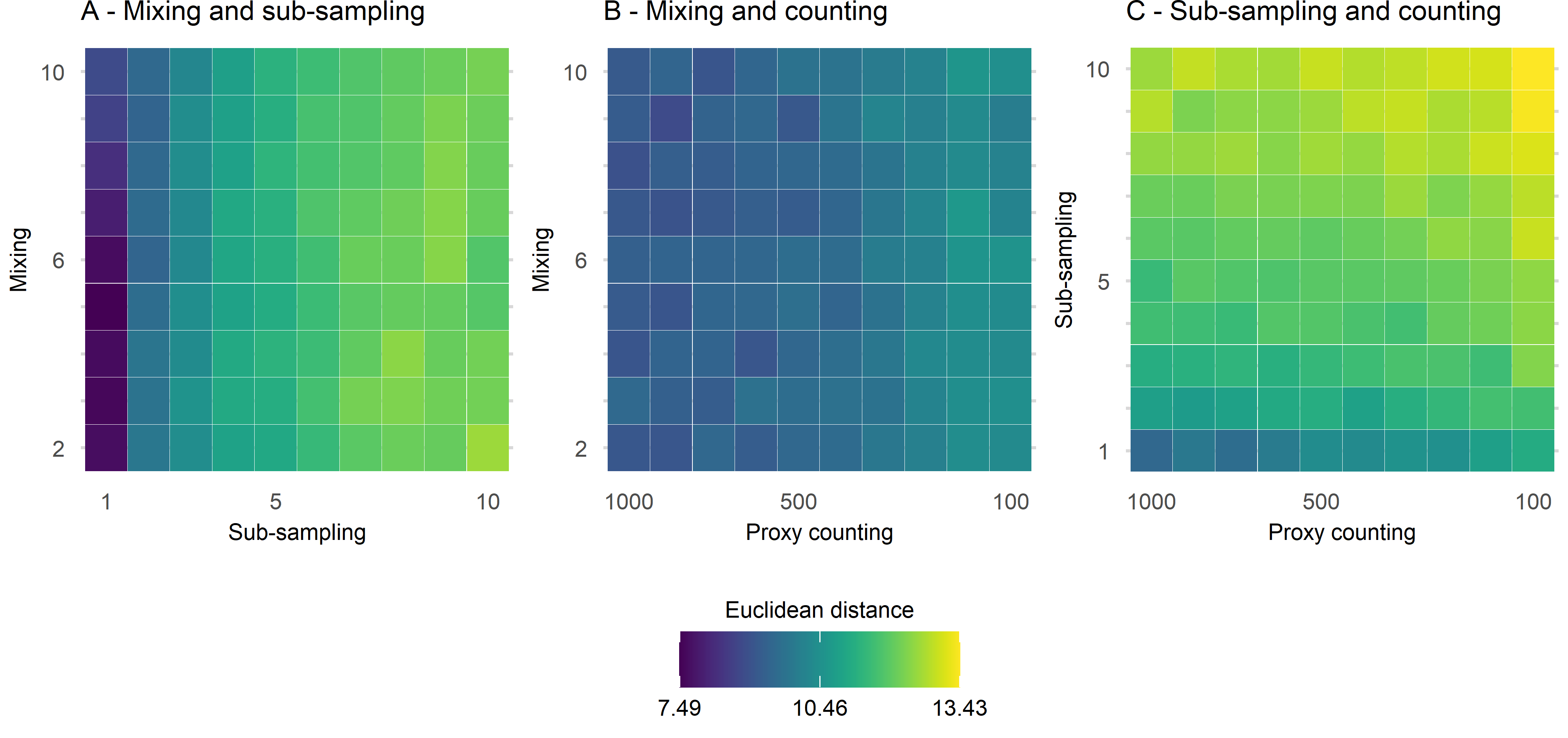
In the following figure (Figure 3), two sources of uncertainty are plotted, one on each axis. What we are interested in here is whether the Euclidean distance increases along the diagonal of the plot, indicating an interaction between the uncertainties. By far the strongest influence is from the combined effect of proxy counting and sub-sampling (Figure 3 C). There appears to be little interaction between mixing and either proxy counting and sub-sampling.
In the main paper, all three uncertainties are combined and visualised. I won’t go there in this short summary! What does this all mean for palaeoecologists?
This approach allows us to make informed decisions around sampling strategies and lab hours spend quantifying proxies. Where should we focus money and effort in a study depending on the research question of interest? We can use this approach to assess how strong the influence of sources of uncertainty are on different statistical methods. Understanding uncertainties is crucial to understanding how reliable our inferences are from the data we have.