Is the past recoverable from the data? Pseudoproxy modelling of uncertainties in palaeoecological data
This paper is about constructing a model that generates patterns of ecological change using population growth equations with underlying dynamics such as threshold points. We show how such a model can be used to assess uncertainties in palaeoecological data using a Virtual Ecological approach. The idea is to generate patterns with the same statistical properties that we see in empirical data, and not to recreate a given ecosystem (i.e., this is a phenomenological model). Why do this? We have no experimental manipulations or direct observations of the long time-scales necessary to understand ecosystem-level change, and even the most highly resolved palaeoecological data from laminated sediment cores contain many uncertainties from environmental processes, sampling, and lab processing. In empirical palaeoecology, we have no ‘known truth’ against which to assess our inferences. By using a virtual ecological approach, we can generate data under ‘known’ conditions.
In reality, we have imperfect knowledge of a perfect world. In simulation, we have perfect knowledge of an imperfect representation of the world.
Why is this all important? Palaeoecological data provide insight into past ecological and climatic change. This source of data is invaluable to understanding ecological change and potential future ecosystem states. However, the data are highly uncertain, relying on many layers of processing such as lab processing, radiocarbon dating, and age depth modelling. The data are often inconsistently spaced through time and may have large time-gaps between observations. Such sources of uncertainty can, at best, mask ‘true’ signals of change, or at worst, lead to false inferences. One way we can assess the influence of uncertainties on statistical inference is through simulation.
If we start with our perfect knowledge of a simulated world, we can also simulate observations from that world, in the same way that we would sample from the real world. This gives us a benchmark dataset, the original simulated data, and a reduced dataset, the sampled simulated data.
Here is my simulated world (Figure 1). Each species on the right (Figure 1 d) is simulated by a population growth equation. The growth rate of each species is their combined response to the two environmental drivers (Figure 1 b). Their optima and tolerance to each driver (Figure 1 c) determine whether the population growth rate of a species is positive or negative. If the environment is unfavourable, then a species population growth rate becomes negative and it will go locally extinct. Species have the chance to re-establish if conditions become favourable again.
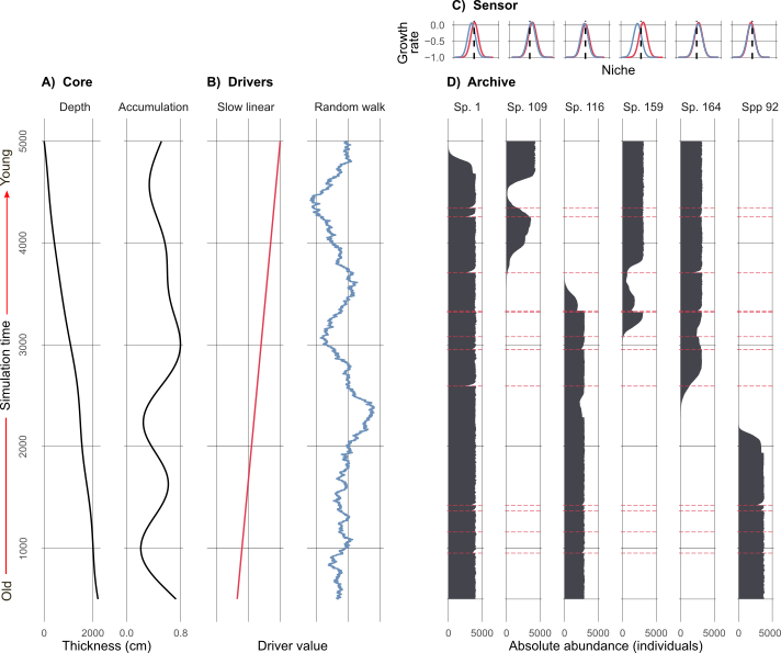
The number of species in (Figure 1) is only a fraction of those simulated. There are actually around 200 potential species, and about 15-40 in existence at any given point in the simulation (depending on the replicate). I simulated a bunch of different driving environments (e.g., one where the environmental driver undergoes an abrupt shift), in the example above (Figure 1) the ‘slow linear’ driver will eventually drive species that existed at the beginning of the simulation locally extinct (unless they were very generalist species!), and new species would establish and thrive.
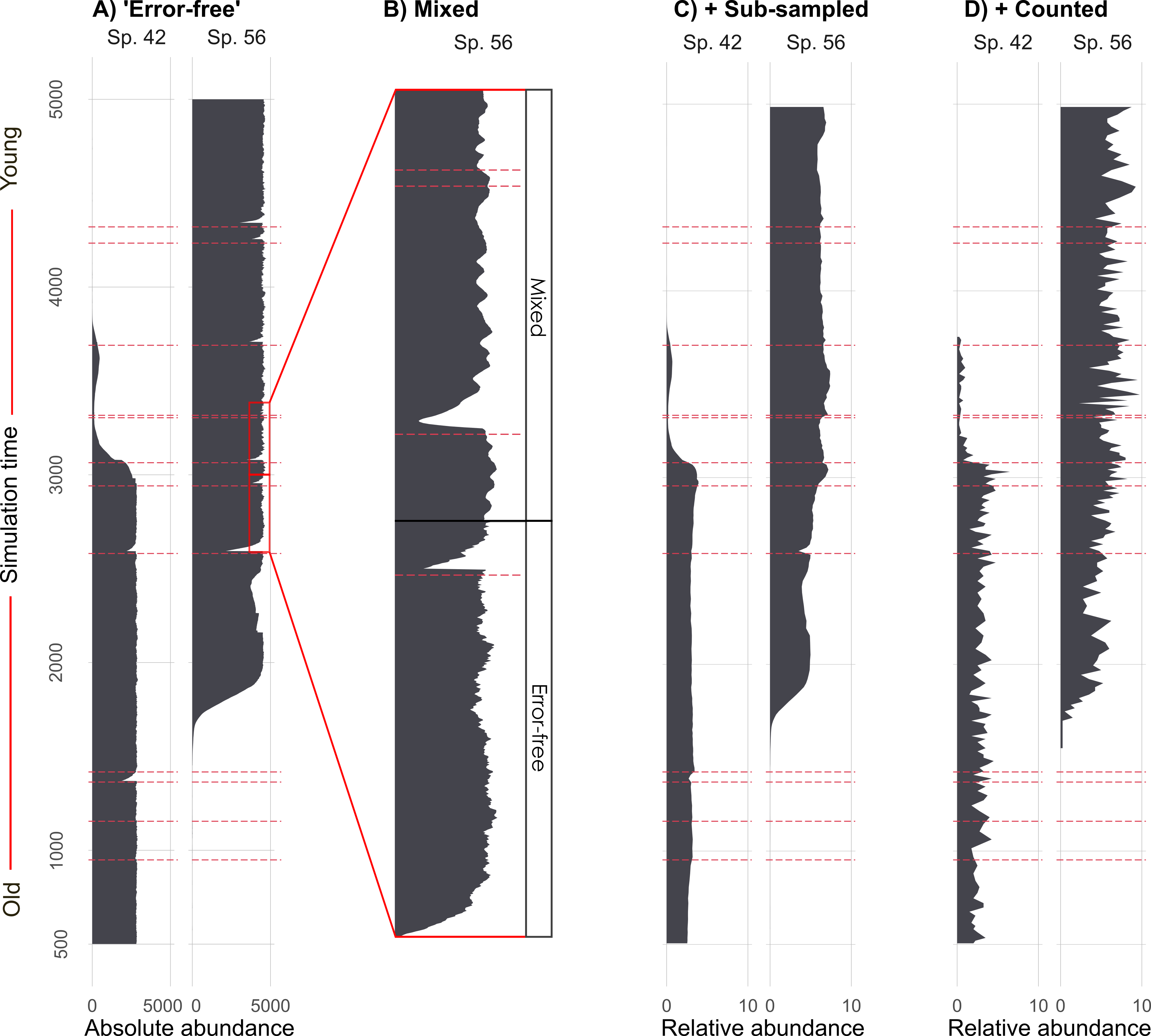
We then take those simulated species abundances (Figure 1 d), remember this is our ‘perfect’ benchmark data, and degrade them with mixing (i.e., a physical process that alters the core), sub-sampling (i.e., slicing up the core into 1 cm segments at given intervals for processing), and proxy counting (i.e., the counting of species under a microscope from the 1 cm segments after lab processing). Figure 2 shows how we start with absolute abundances of species, and recreate the observational process, ultimately resulting in data that look a lot more like what we see in reality from proxy-data.
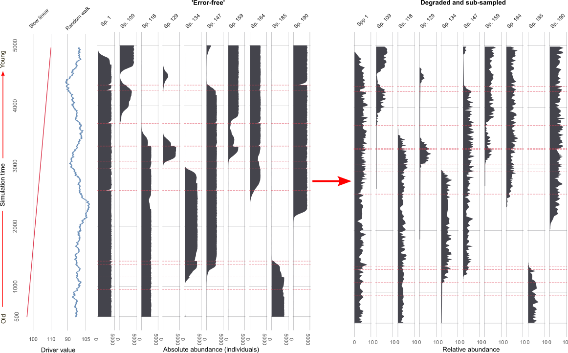
This is what a larger subset of the simulated species looks like before and after the virtual degradation and sub-sampling process (Figure 3).
Finally, we analyse both sets of data. In simulation the three sources of uncertainty (mixing, sub-sampling, and proxy counting) are applied individually, and in combination, at increasing levels of severity. So we end up with 1210 (per simulation replicate!) datasets from the ‘error-free’ benchmark to the most degraded. We analyse them all! But here is an example of the benchmark, and one level of degradation (Figure 4).
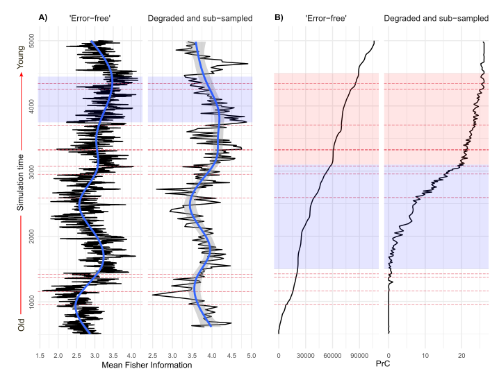
This figure shows two different multivariate community analyses (Fisher Information and principal curves), and how the results change between the ‘error-free’ data and the degraded and sub-sampled dataset. At the start, I mentioned that uncertainty can lead to incorrect inference. This example is only of one randomly selected model replicate, but it shows how interpretations can be influenced by uncertainties. The 700 year-long period of reversed directionality in Fisher Information (Figure 4 A) can change our inference from a system increasing in stability, to decreasing in stability (a decrease in Fisher Information is interpreted as a system becoming less predictable less stable). The principal curve changing from a gradual increase (a good representation of change driven by the primary driver system), to a sigmoidal shape (Figure 4 B), can alter our interpretation of the ‘true’ rate of species turnover in the system. This example demonstrates well how a Virtual Ecological approach can be used to assess uncertainty and its influence on statistical inference.