Authoring collaborative research projects using Quarto

Quinn Asena

UW-Madison

2024-07-07

Quarto for collaborative research

Link to slides

why geek out on Quarto?

why I like Quarto

  • Well documented

  • Uses markdown syntax

  • Accepts multiple programming languages

  • Outputs multiple formats (Word, PDF, HTML…)

  • Easy to learn and transfer skills from other languages

another thing to learn?

  • R Markdown and Jupyter also support multiple languages too…

  • You decide ʕ•́ᴥ•̀ʔっ

  • What you learn here is generalisable!

XKCD nails it again!

why collaborate via Quarto and Git?

  • Version control your projects

  • Generate a citable DOI and use for supplimentary information

  • Reproducibility: whole workflow from data to results in one place

  • Host a live link consistent with current results (no more copy paste 7 plots into a word doc each time you change something!)

  • Coding colaborators can contribute via a Git workflow

  • Communicate results to non-coding collaborators

How does it work? Commandline vs code editor:

  • Quarto is commandline, and VS Code and RStudio are editors

Quarto uses knitr for R and Jupyter for Python

Buckle up, ready your coding fingers!

today’s goals

  • Learn the necessary components of a Quarto document to publish an HTML

  • Publish an example link on GitHub

  • Have a working template you can use in the future

  • Know where to find help and useful resources

Zoom

  • Camera optional, but we love to see you (really, it helps me a lot!)

  • During exercises, give me a ✔️ when you are done or a if you need help

  • Drop questions in the Zoom chat or raise a hand at any time

first things first

It sometimes takes a minute for GitHub to host your repo, so let’s get this process underway.

GitHub

  • Go to the session repo

  • Fork the repository

  • Settings -> GitHub pages -> enable github pages

  • By default, your link will be hosted at: https://githubusername.github.io/reponame/pathtodocument.html

  • The repo can remain private but anyone who has the link can view it.

Let’s code!

We are using VS Code, R, and GitHub. If you have a preferred workflow like RStudio, Python, or GitKraken you can use them but may be harder to follow the session content. Afterall, Quarto is supposed to be flexible!

GitHub

  • Open up VS Code and navigate to the source control

    • Clone https://github.com/username/resbaz2022
  • Open up the install.R and template.qmd files

    • Run the install file, then render the template

elements of a Quarto file

  • YAML

  • Text

  • Code blocks

  • References file

  • scss (optional for style; won’t cover this!)

YAML

The YAML is a set of key: value pairs that are the metadata for your document, such as, author, title, output format, and citation file.

  • YAML is whitespace sensitive
  • Indent sensitive
  • Can be a separate file named _quarto.yml
---
title: "My Manuscript"
format: html
date: today
---

YAML exercise

Your Turn 💻 :

YAML exersice

  • Open up the template.qmd and fill the title: and name: and affiliation: fieds.

    • A couple of handy entries are already completed

    • The existing field: date: today will automatically generate today’s date (cool huh? ͡▀̿ ̿ ͜ʖ ͡▀̿ ̿ )

  • Add a table of contents following the guide

  • Render the document

  • Give me a ✔️ when done or a if you need help

text editing

  • Writing in Quarto uses markdown syntax

  • LaTeX is used to render PDFs so LaTeX commands can be used for PDF outputs

  • Look! I can do fancy maths: \(f_{c}=z^{2}+c\)

    • ▀̿ ̿ ͜ʖ ͡▀̿ ̿

Pro tip!

Render regularly. Small errors can be tricky to pick out long after they have been made.

You can change the defult so that the document renders on hitting save.

including a bibliography

Citations require:

  • a .bib or .bibtex file in your working directory (one is included for today)

    • The references file can be generated (and automatically sync) with Zotero and other reference managers.
  • a YAML entry pointing to the file bibliography: refs.bib (if the file is named ‘refs.bib’)

  • an optional CSL file specifying the format of the bibliography.

Pro tip!

There are alternative methods that do not require a local file, like CiteDrive.

in-text citations

Citing work in-text follows the @citekey format

  • @perkel2022 = Perkel (2022)

  • [@chamberlin1897; @perkel2022] = (Chamberlin 1897; Perkel 2022)

  • Quarto, by default, inserts a formatted reference list at the end of the document so I put an empty ‘References’ header.

We won’t go deeper into citations for now as we are not authoring an article today. The link above has info for technical writing.

equations

Pretty, formatted equations can be inserted using the same syntax as in LaTeX. Inline equations (e.g., \(E = mc^2\)) are surrounded by a $ and equation bocks are surrounded by $$:

\[ N_{t+1} = N_t + r_{d}N_t \left(1- \frac{N_t}{K} \right) \]

handy features

The RStudio IDE has some handy features using the visual editor:

VS Code also has cool features:

markdown exercise

Your Turn 💻 :

Markdown exercise

In the template Introduction section take 3-4 minutes to write:

  • a sub-heading under the introduction

  • a list

  • and an equation

  • cite one of the articles in in existing .bib file using the @

  • render the document and hit the ✔️ in zoom

code blocks

Code is executed when the document is rendered. Code blocks can also be executed individually just like regular R markdown if you are already familiar with that. Code blocks are inserted like this:

```{r}
6*7
```
[1] 42

code block execution option

Code block execution options options are set with a special comment: #| (white space sensitive!). Block options determine how the code is executed, e.g., whether to display the code block: #| echo: true, warning messages #| warning: false, and to input captions #| fig-cap: "A really good figure caption!".

Pro tip!

Unlike R markdown, block options are lower case true/false and the comment #| must be followed by a space.

document level execution option

Execution options can also be set at the document level under the YAML entry execute::

execute:
  echo: false
  warning: false
format: 
  html:
    fig-width: 8
    fig-height: 6
  pdf:
    fig-width: 7
    fig-height: 5

inline code

Code can also be executed inline:

Seven times six is `r 7 * 6`

Inline code execution can be helpful referencing values in text like: there are nrow(data) observations in the data.

code exercise

Your Turn 💻 :

Code block exercise

  • Check out the execution options and edit the existing code block options in the ‘Libraries section’ to:

  • exclude the results

  • exclude displaying the code (make sure it still evaluates!)

  • render the document and hit the ✔️ in zoom

cache

Cache keeps a record of outputs and only re-runs code chunks that have beed edited. Caching is useful for computations that take a long time and do not need to be re-run every time you render the document. Cache can be set at the document level using the YAML entry:

execute:
  cache: true

or using the ececution option #| cache: true in an individual code block.

Nap time (not really…)!

Refil on tea, coffee, and cookies.

tables

tabsets

Ok now the feature I find very useful: tabsets. Tabsets are great for showing, multiple results, data, code, whatever you want in tabs. Say, you want to show the plot on one tab and the model output table in the next, or multiple related plots. Much easier to read and flick among results than a long stream of plots and tables.

if (!require("pacman")) install.packages("pacman", repos="http://cran.r-project.org")
pacman::p_load(ggplot2, palmerpenguins)    # Install & load packages
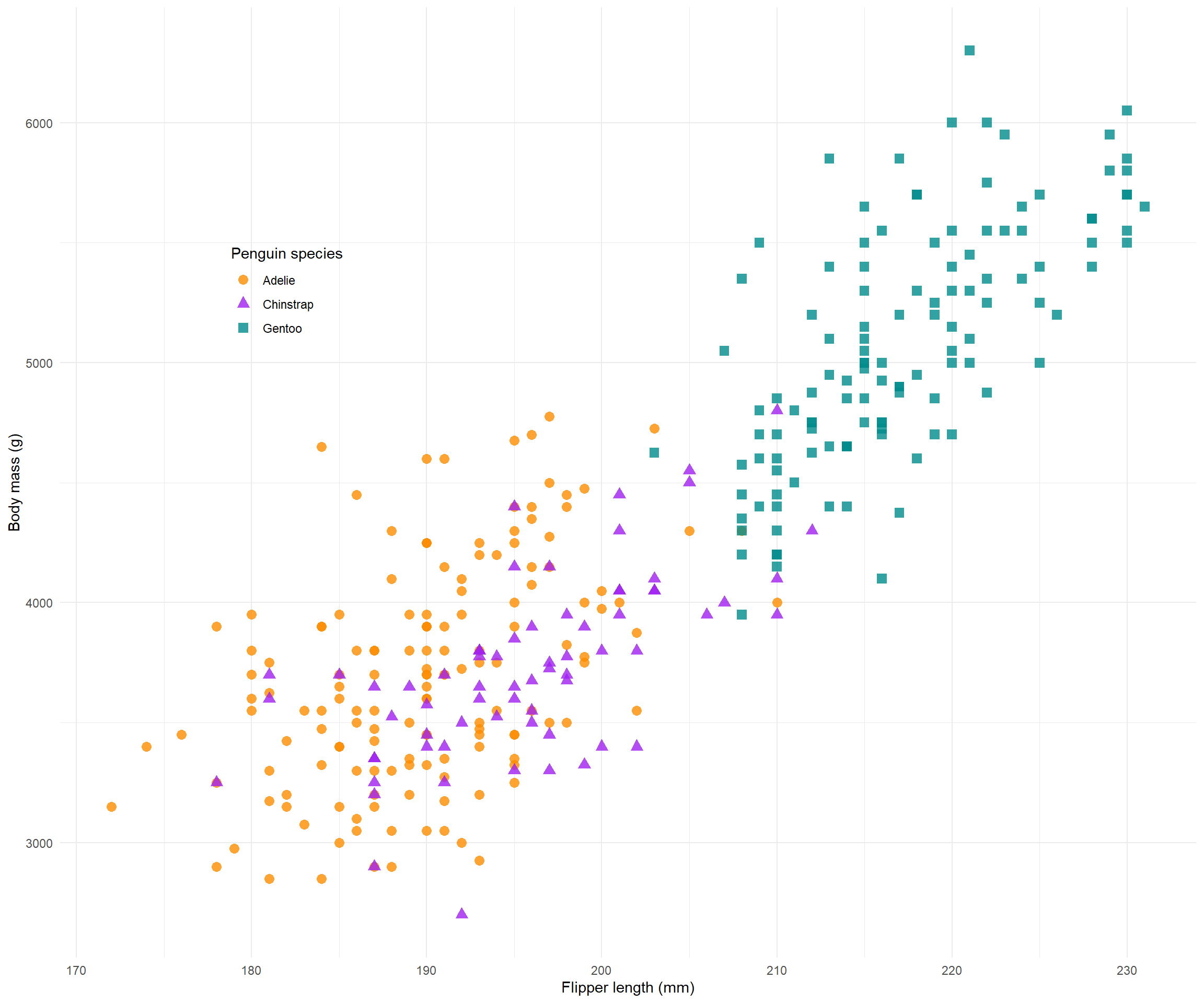
# From: https://allisonhorst.github.io/palmerpenguins/articles/examples.html
mass_flipper <- ggplot(data = penguins,
                       aes(x = flipper_length_mm,
                           y = body_mass_g)) +
  geom_point(aes(color = species,
                 shape = species),
             size = 3,
             alpha = 0.8) +
  scale_color_manual(values = c("darkorange","purple","cyan4")) +
  labs(x = "Flipper length (mm)",
       y = "Body mass (g)",
       color = "Penguin species",
       shape = "Penguin species") +
  theme_minimal() +
  theme(legend.position = c(0.2, 0.7),
        plot.title.position = "plot",
)

Plot of penguin bill length against body mass by species

Flipper length and body mass for Adelie, Chinstrap and Gentoo Penguins from Allison Horst

tabset code

Your Turn 💻

Tabsets are created with the following syntax:

:::{.panel-tabset}
# Tab 1
content

# Tab 2
content
:::

Tabset exercise

  • Check out the tabset panel documentation

  • Create a tabset with three tabs in the template under the Tabsets heading

    • Does not matter what they contain but feel free to blurb something in there
  • render the document and hit the ✔️ in zoom

images

Figures can be generated directly from code (as in the tabset panel demonstration) or inserted as files using the ![caption](pathway/to/img) syntax (for more details like multi-figure layot and alt text see: figures in Quarto).

Images exercise

  • There is a (royalty free) XKCD comic inside the images directory in the repo. using the syntax described above, insert the image into one of the tabsets you just created.

  • render the document and hit the ✔️ in zoom

let’g go Git it

You’re now ready to host your live link!

GitHub

  • Render your project so that most recent changes are exported

  • In the source control on the left commit and push your changes

    • You can do this however you prefer, commandline, GUI, source control…
  • Find your hosted template link and share with the world!

Congrats you did it (ง ͡❛ ͜ʖ ͡❛)ง

how did I do?

Before you go! Please post in the chat:

  • a one up (a good thing)

  • and one down (a bad thing)

or email me at qasena@wisc.edu

References

Biostats - very useful resource for authoring documents in Quarto. This session draws from their content.

Awsome Quarto - a big list of Quarto things.

Chamberlin, T. C. 1897. “The Method of Multiple Working Hypotheses.” The Journal of Geology 5: 837–48.
Perkel, Jeffrey M. 2022. “Cut the Tyranny of Copy-and-Paste with These Coding Tools.” Nature 603 (7899): 191–92. https://doi.org/10.1038/d41586-022-00563-z.