multinomialTS Vignette

Introduction

One of the primary goals of this model is to be able to test multiple hypotheses about the data and lend statistical support to the different hypotheses. For example which environmental drivers are having the strongest effects on which taxa? Or, are interactions among taxa or abiotic variables driving change in the system? This state-space approach allows us to estimate coefficients for taxa interactions and driver-taxa relationships, that we don’t get from methods such as ordination or cluster analysis. We recommend this method as complimentary to other methods, as both have their advantages.

This vignette

This vignette will take us through:

Choosing a prediction resolution for mnTS() (Section 2).
The fitting process (Section 3).
- Finding initial conditions with mnGLMM() (Section 3.1).
- Fitting mnTS() with and without species interactions (Section 3.3).
Assessing the resulting models (Section 3.4).

Data processing

This vignette will work with the data that have focal taxa and groups already wrangled. A second vignette will be added to cover the data wrangling, for now see this workshop

# Load required packages
library(ggplot2)
library(dplyr)
library(tidyr)
library(stringr)
library(scales)
library(RcppArmadillo)
library(minqa)
library(matrixStats)
library(numDeriv)
library(mvtnorm)
library(multinomialTS)

# Read-in the wrangled data 
# Read in our X variables
data("story_char_wide", package = "multinomialTS")
# Read-in the long data for plotting
data("story_pollen_wide", package = "multinomialTS")
# Read-in bootstrapped model
data("story_100_bootstraps", package = "multinomialTS")

Here is what the state variable ( $Y$ ) data look like:

head(story_pollen_wide)

# A tibble: 6 × 7
# Groups:   age, depth [6]
     age depth other hardwood `Fagus grandifolia` Quercus Ulmus
   <dbl> <dbl> <int>    <int>               <int>   <int> <int>
1 -66.2    0.5   106       60                   8      96     9
2   2.85  32.5   169       26                   8      59    10
3  45.8   64.5   189       27                   8      58     7
4  94.1   96.5   209       17                   2      42    17
5 191.   128.    161       34                  13      55    20
6 203.   132.     88       52                  34      91    19

And our covariate ( $X$ ):

head(story_char_wide)

# A tibble: 6 × 3
    age depth char_acc
  <dbl> <dbl>    <dbl>
1 -66.2   0.5      0
2 -63.4   1.5     15.8
3 -61.4   2.5     40.3
4 -59.8   3.5     21.8
5 -58.5   4.5     37.3
6 -57.2   5.5     29.8

For the moment, we are keeping the age and depth columns in both tibbles. These columns are so that we have a common variable to match the two tibbles, and will be removed a little later.

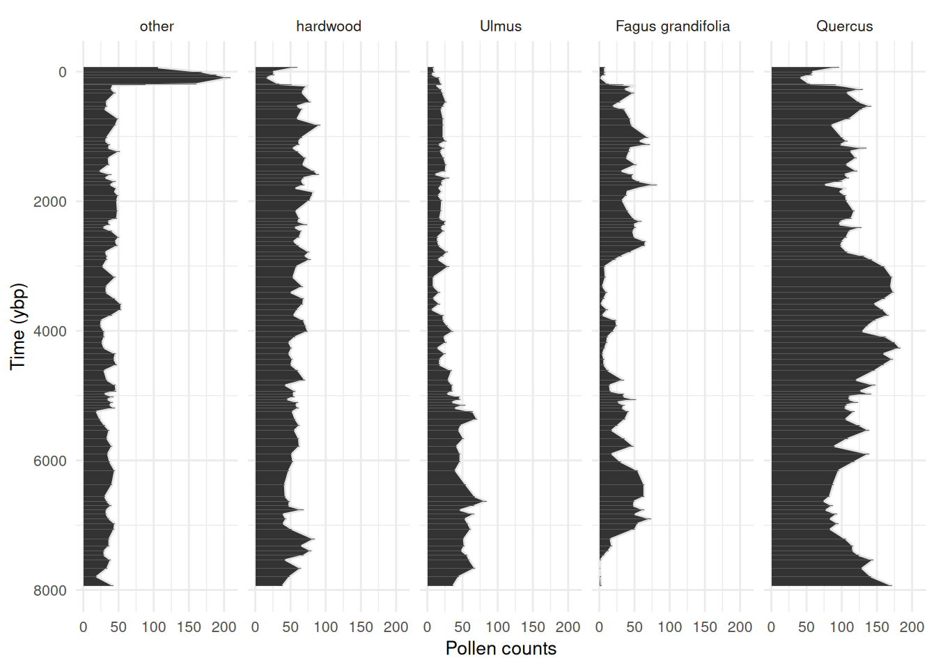
Always check out some plots! See that big spike in “other”, this is the rise of ambrosia in recent decades. Worth clipping that from the data, major trends in the out-group indicates that something important is being aggregated in the reference (we don’t want that). I have left it in this example dataset for demonstration purposes.

Code

story_pollen_wide |>
  pivot_longer(-c(age, depth)) |>
  mutate(name = factor(name,levels = c(
    "other", "hardwood", "Ulmus", "Fagus grandifolia", "Quercus"))) |>
  ggplot(aes(x = age, y = value)) +
    geom_area(colour = "grey90") +
    geom_col() +
    scale_x_reverse(breaks = scales::breaks_pretty(n = 6)) +
    coord_flip() +
    labs(y = "Pollen counts", x = "Time (ybp)") +
    facet_wrap(~name,
               nrow = 1) +
    theme_minimal() +
    theme(
      text = element_text(size = 10)
    )

State variables $Y$

We will start off by choosing a resolution for the model predictions (e.g., predicting ecological process at 50 or 100 year intervals).

# Time-span of the data divided by the number of observations
max(story_pollen_wide$age) / nrow(story_pollen_wide)

[1] 83.48578

# Age differences between successive observations
diff(story_pollen_wide$age)

 [1]  69.017  42.946  48.331  96.968  11.459  14.340  54.308  55.284 138.681
[10]  66.118  48.695 143.230 103.015 186.753  58.537  54.550  52.888  50.954
[19] 104.623 100.248 100.144  51.406  53.372  52.350  53.950  51.957  53.782
[28]  59.512  72.266 168.719 111.125  47.302  47.531  47.949  55.391  90.190
[37]  66.359  68.199  97.921  60.144  54.207 109.400 165.792 141.147  93.284
[46]  90.969  85.959  87.634  86.346  79.080  85.733  84.658  85.647  85.731
[55]  86.000  88.257  84.158  86.849  90.252 144.587  79.708  89.321  43.635
[64]  43.511  42.991  42.250  44.523  47.083  54.088 115.201  99.857  73.484
[73] 128.326 116.359 119.324 123.707 132.304 219.725 184.122  71.101  68.843
[82]  66.205  65.555  71.999  71.922  86.020 153.328 103.854  76.139  71.061
[91]  71.132 129.632 127.729 137.070

# The range of the age differences
range(diff(story_pollen_wide$age))

[1]  11.459 219.725

# the average of the age differences
mean(diff(story_pollen_wide$age))

[1] 85.0778

sd(diff(story_pollen_wide$age))

[1] 38.36777

This all looks great! If we bin the data at around 50-75 years, we will still have most of our data in independent bins.

Now that we know roughly what bin-width to use to maximize the number of observations in the state variables, we will apply the same bin-width to both the state variables and the covariate data.

Handling the covariates $X$

Covariates need to be handled according to decisions that were made around the state variables, that is, if the state variables were binned at a century-level resolution then the covariates must match that resolution. We can have a finer temporal resolution of the covariates than we do of the state variables. In this dataset, our state variables have 95 observations, and our covariate has 646 observations over the same time-span. Having more observations of environmental covariates is common in palaeo-data and works well with fitting the model.

Since we need to apply the same binning procedure to both the state variables and the covariate, I like to join both datasets. Charcoal was sampled to a greater depth than the pollen data, so we are going to clip the covariate to the extent of the state variables and join the two datasets by their common variable, age.

# Clip covariate data to the extent of the state variables
# Join the two by age so that we get a square matrix
story_join <- story_char_wide |>
  dplyr::filter(age <= max(story_pollen_wide$age)) |>
  left_join(story_pollen_wide)

# Always double check dimensions before/after joining!
# dim(story_join)
# tail(story_join)

Now we have all our data joined. Note that the covariate $X$ (char_acc) has observations every cm, whereas pollen was sampled at less frequent intervals (this is OK!).

head(story_join, n = 10)

# A tibble: 10 × 8
     age depth char_acc other hardwood `Fagus grandifolia` Quercus Ulmus
   <dbl> <dbl>    <dbl> <int>    <int>               <int>   <int> <int>
 1 -66.2   0.5     0      106       60                   8      96     9
 2 -63.4   1.5    15.8     NA       NA                  NA      NA    NA
 3 -61.4   2.5    40.3     NA       NA                  NA      NA    NA
 4 -59.8   3.5    21.8     NA       NA                  NA      NA    NA
 5 -58.5   4.5    37.3     NA       NA                  NA      NA    NA
 6 -57.2   5.5    29.8     NA       NA                  NA      NA    NA
 7 -56.0   6.5    34.4     NA       NA                  NA      NA    NA
 8 -54.8   7.5    21.2     NA       NA                  NA      NA    NA
 9 -53.7   8.5    20.5     NA       NA                  NA      NA    NA
10 -52.6   9.5     8.26    NA       NA                  NA      NA    NA

I always do lots of quick checks like head(), tail(), dim() (and many more!) to make sure to catch any coding mistakes!

tail(story_join, n = 10)

# A tibble: 10 × 8
     age depth char_acc other hardwood `Fagus grandifolia` Quercus Ulmus
   <dbl> <dbl>    <dbl> <int>    <int>               <int>   <int> <int>
 1 7777.  648.     2.50    NA       NA                  NA      NA    NA
 2 7794.  648.     8.19    19       49                   2     142    45
 3 7812.  650.    19.1     NA       NA                  NA      NA    NA
 4 7829.  650.     6.19    NA       NA                  NA      NA    NA
 5 7845.  652.     2.78    NA       NA                  NA      NA    NA
 6 7863.  652.     4.20    NA       NA                  NA      NA    NA
 7 7880.  654.     5.02    NA       NA                  NA      NA    NA
 8 7898.  654.     3.17    NA       NA                  NA      NA    NA
 9 7914.  656.     4.51    NA       NA                  NA      NA    NA
10 7931.  656.     2.60    43       39                   3     172    37

This all looks good, and we can now bin the data to an appropriate temporal resolution for fitting the model. Choosing a bin-width may take some trial and error, I’m going with a bin-width of 50 years.

# This code chunks the data into bins and gives us a grouping variable "bins"

bin_width <- 50
bins <- cut(story_join$age,
            breaks = seq(from = min(story_join$age),
            to = max(story_join$age + bin_width),
            by = bin_width), include.lowest = TRUE, labels = FALSE)

We now apply the bins to our data. For most types of covariates we want the average value of the covariate in each bin. But for the pollen count data, we want the sum. This is because of the underlying multinomial distribution in the model.

# Assign bin indices, then summarise: mean age and charcoal per bin; sum pollen counts per bin
story_binned <- bind_cols(bins = bins, story_join) |>
  group_by(bins) |>
  summarise(
    age = mean(age, na.rm = T), # the center of the bin
    char_acc = mean(char_acc, na.rm = T), # mean charcoal accumulation rate per bin
    other = sum(other, na.rm = T), # the sums of the count data
    hardwood = sum(hardwood, na.rm = T),
    `Fagus grandifolia` = sum(`Fagus grandifolia`, na.rm = T),
    Ulmus = sum(Ulmus, na.rm = T),
    Quercus = sum(Quercus, na.rm = T)
  ) |>
  arrange(desc(age))
# Be aware that the gaps in the pollen data are now filled with 0's not NA

This is important

We want the model to run from the past to the present, and the model runs from the top of the matrix to the bottom. So we want to make sure that the top row of the data is the oldest date. Palaeo-data are usually ordered from the top of the core to the bottom (present to past), so we arrange(desc(age)).

Let’s see what the data look like binned at a 50 year resolution:

head(story_binned, n = 10)

# A tibble: 10 × 8
    bins   age char_acc other hardwood `Fagus grandifolia` Ulmus Quercus
   <int> <dbl>    <dbl> <int>    <int>               <int> <int>   <int>
 1   160 7914.     3.43    43       39                   3    37     172
 2   159 7863.     4.00     0        0                   0     0       0
 3   158 7812.    11.1     19       49                   2    45     142
 4   157 7761.     4.06     0        0                   0     0       0
 5   156 7713.     5.29     0        0                   0     0       0
 6   155 7666.     8.24    34       65                   1    68     129
 7   154 7609.     8.50     0        0                   0     0       0
 8   153 7553.     9.27    39       43                   2    60     145
 9   152 7502.     5.05     0        0                   0     0       0
10   151 7457.     5.46    30       69                   7    57     125

This is looking good, we have reduced the time-intervals over which to iterate the model. The data are now 160 rows with complete covariate data, containing 93 state variable observations. The original number of pollen observations was 95, so we have not summed many observations within the same bins.

multinomialTS requires two matrices, a site-by-species matrix $Y$ , and a covariate matrix $X$ , so we will leave tibbles behind and split the data. $X$ variables may be of different types (e.g., continuous, categorical…) but should be scaled relative to each other.

story_pollen_matrix <- story_binned |>  # Select taxa
  select(other, hardwood, Ulmus, `Fagus grandifolia`, Quercus) |> 
  rename("Fagus" = "Fagus grandifolia") |> 
  as.matrix()
# Replacing 0 with NA is not strictly necessary the way we use the data today
# But it is a good safety to avoid 0-count data where it should be no observation
story_pollen_matrix[which(rowSums(story_pollen_matrix) == 0), ] <- NA
head(story_pollen_matrix)

     other hardwood Ulmus Fagus Quercus
[1,]    43       39    37     3     172
[2,]    NA       NA    NA    NA      NA
[3,]    19       49    45     2     142
[4,]    NA       NA    NA    NA      NA
[5,]    NA       NA    NA    NA      NA
[6,]    34       65    68     1     129

story_char_matrix_scaled <- story_binned |> # select covariates
  select(char_acc) |> 
  as.matrix() |> 
  scale() # Scale covariates
head(story_char_matrix_scaled)

       char_acc
[1,] -0.9826414
[2,] -0.8978991
[3,]  0.1548837
[4,] -0.8894600
[5,] -0.7078643
[6,] -0.2731469

Fitting `multinomialTS`

OK, now we have:

Chosen a temporal resolution for the model of 50-year bins
Organised the data into a site-by-species matrix $Y$ at 50-year bins
Binned and scaled covariate matrix $X$

With that, we can fit the model.

Finding initial conditions using `mnGLMM()`

The mnTS() function will provide estimates for biotic interactions ( $C$ matrix), taxa-driver relationships ( $B$ matrix), and cross-correlated error ( $V$ matrix). But the model needs initial starting values for these parameters to begin with. We get initial starting conditions from the data by running the mnGLMM() function. mnGLMM() returns estimates for the $B$ and $V$ matrices (not the $C$ matrix) and assumes that there are no time gaps in the data.

Tip

The arguments of the starting values in both the mnGLMM() and mnTS() are all suffixed with .start (e.g., B.start will be the starting values for the $B$ matrix).

The arguments of the parameters to be estimated are all suffixed with .fixed (e.g., B.fixed will be parameters that are estimated from $B$ matrix).

Setting-up parameters for `mnGLMM()`

Now, lets set up the parameters for mnGLMM(). We need:

A vector that indicates the row indices where there are state variable observations: sample_idx
An integer number of covariates (+ 1 for mnGLMM()): p
An integer of the number of state variables: n
A matrix of starting values for $B$ : B.start.glmm
A matrix of $B$ parameters to estimate: B.fixed.glmm
A matrix of $V$ parameters to estimate: V.fixed.glmm

# Row indices of non-empty time bins (bins containing at least one pollen observation)
sample_idx <- which(rowSums(story_pollen_matrix) != 0)
# Verify: all rows should have non-zero counts
head(story_pollen_matrix[sample_idx, ])

     other hardwood Ulmus Fagus Quercus
[1,]    43       39    37     3     172
[2,]    19       49    45     2     142
[3,]    34       65    68     1     129
[4,]    39       43    60     2     145
[5,]    30       69    57     7     125
[6,]    30       80    49    13     116

Set-up the remaining parameters:

# p = number of covariates + intercept; n = number of taxa
p <- ncol(story_char_matrix_scaled) + 1
n <- ncol(story_pollen_matrix)
# Estimate all diagonal variances; fix reference taxon variance (V[1,1]) to 1 for identifiability
V.fixed.glmm <- diag(n)
diag(V.fixed.glmm) <- NA
V.fixed.glmm[1] <- 1
# Fix reference taxon (column 1) coefficients to 0; estimate all others (NA = estimate)
B.fixed.glmm <- matrix(c(rep(0,p),rep(NA, (n - 1) * p)), p, n)
B.start.glmm <- matrix(c(rep(0,p),rep(.01, (n - 1) * p)), p, n)

These parameters are used as arguments to the mnGLMM() function. Check them out by printing them in your console. Each matrix needs to be the correct dimensions given the number of taxa and number of covariates. The position elements of each matrix reflect the species and/or the covariates, as we will see later in the output of the model.

Fitting `mnGLMM()`

Remember that mnGLMM() does not handle gaps in the data and only fits complete $X$ and $Y$ matrices. We have created a variable for our observation indices (sample_idx), so for mnGLMM() we will index the matrices by this variable: e.g., story_pollen_matrix[sample_idx, ].

# fit glmm
start_time <- Sys.time()
glmm_mod <- mnGLMM(Y = story_pollen_matrix[sample_idx, ],
                   X = story_char_matrix_scaled[sample_idx, ,drop = F],
                   B.start = B.start.glmm,
                   B.fixed = B.fixed.glmm,
                   V.fixed = V.fixed.glmm)
end_time <- Sys.time()

I like to keep track of how long the models take to run. This will vary depending on the data set and the system hardware, but can be useful benchmarking for running models repeatedly. Note the time increase as we progess from mnGLMM() to mnTS() without, and then with interactions.

end_time - start_time

Time difference of 12.72835 secs

The outputs of mnGLMM() can be examined with the summary(glmm_mod) function.

summary(glmm_mod)


Call: mnGLMM with Tmax =  93  n =  5

logLik = 506.1927,  AIC = -984.3855 [df = 14]

dispersion parameter =  1

Fitted Coefficients with approximate se
                           Coef.         se          t            P
(intercept).hardwood  0.32520750 0.08449716  3.8487389 1.187275e-04
char_acc.hardwood    -0.15611319 0.08828448 -1.7682971 7.701124e-02
(intercept).Ulmus    -0.31412746 0.11063702 -2.8392617 4.521805e-03
char_acc.Ulmus       -0.27877439 0.10904240 -2.5565689 1.057101e-02
(intercept).Fagus    -0.26463088 0.11061642 -2.3923292 1.674182e-02
char_acc.Fagus       -0.44517937 0.11465590 -3.8827428 1.032848e-04
(intercept).Quercus   0.99820757 0.08800696 11.3423709 8.092196e-30
char_acc.Quercus     -0.06223225 0.09098385 -0.6839923 4.939800e-01


Overall model

B =
            other   hardwood      Ulmus      Fagus     Quercus
(intercept)     0  0.3252075 -0.3141275 -0.2646309  0.99820757
char_acc        0 -0.1561132 -0.2787744 -0.4451794 -0.06223225

sigma =  1.055386

V =
         other    hardwood     Ulmus     Fagus    Quercus
other        1 0.000000000 0.0000000 0.0000000 0.00000000
hardwood     0 0.004430489 0.0000000 0.0000000 0.00000000
Ulmus        0 0.000000000 0.3021321 0.0000000 0.00000000
Fagus        0 0.000000000 0.0000000 0.3045221 0.00000000
Quercus      0 0.000000000 0.0000000 0.0000000 0.07575794

Setting-up parameters for `mnTS()`

Now, lets set up the parameters for mnTS(). mnTS() needs:

row indices as before: sample_idx
the number of covariates: p
the number of state variables: n
starting values for each matrix:
- $B0$ : B0.start.mnTS (intercept)
- $B$ : B.start.mnTS (driver-taxa)
- $C$ : C.start.mnTS (taxa interactions)
- $V$ : V.start.mnTS (cross-correlated error)
parameters to estimate for each matrix:
- $B0$ : B0.fixed.mnTS
- $B$ : B.fixed.mnTS
- $C$ : C.fixed.mnTS
- $V$ : V.fixed.mnTS

We are using the output from mnGLMM() as starting values for the matrices $B0$ , $B$ , and $V$ . mnGLMM() does not provide estimates for $C$ , so we handle $C$ a little differently and we input values close to zero for each parameter estimated and let mnTS() do the rest.

# Use GLMM estimates as starting values for mnTS: row 1 = intercepts, row 2 = covariate slopes
B0.start.mnTS <- glmm_mod$B[1, , drop = F]
B.start.mnTS <- glmm_mod$B[2, , drop = F]

# Allow all V elements to be estimated; fix reference taxon variance V[1,1] to 1 for identifiability
V.fixed.mnTS <- matrix(NA, n, n)
V.fixed.mnTS[1] <- 1

V.start.mnTS <- glmm_mod$V  # initialise V from GLMM estimate

# Fix reference taxon (column 1) B coefficients to 0; fix reference taxon intercept to 0
B.fixed.mnTS <- matrix(NA, p-1, n)
B.fixed.mnTS[,1] <- 0
B0.fixed.mnTS = matrix(c(0, rep(NA, n - 1)), nrow = 1, ncol = n)

# Diagonal-only C matrix: self-regulation terms only, no between-taxon interactions
# NA = estimate; 0 (off-diagonals) = fixed at zero
C.start.mnTS  <- .5 * diag(n)
C.fixed.mnTS <- C.start.mnTS
C.fixed.mnTS[C.fixed.mnTS != 0] <- NA

Fitting `mnTS()`

Remember, mnTS() does handle gaps in the state-variables where there are data in the covariate matrix. In the following code, we use the complete (no gaps) $Y$ matrix story_pollen_matrix[sample_idx, ] with dimensions: 93, 5. And the full $X$ matrix: story_char_matrix_scaled with dimensions: 160, 1. We will fit the model twice:

Without taxa interactions.
With taxa interactions.

Tip

Note the use of sample_idx in story_pollen_matrix[sample_idx, ] and Tsample = sample_idx. This is important as it tells the model where there are observations of $Y$ in relation to observations in $X$ .

start_time <- Sys.time()
mnTS_mod <- mnTS(Y = story_pollen_matrix[sample_idx, ],
                 X = story_char_matrix_scaled, Tsample = sample_idx,
                 B0.start = B0.start.mnTS, B0.fixed = B0.fixed.mnTS,
                 B.start = B.start.mnTS, B.fixed = B.fixed.mnTS,
                 C.start = C.start.mnTS, C.fixed = C.fixed.mnTS,
                 V.start = V.start.mnTS, V.fixed = V.fixed.mnTS,
                 dispersion.fixed = 1, maxit.optim = 1e+6)
# maxit.optim is the max number of iterations the optimiser will complete before stopping.
# increase maxit.optim if the model needs a lot of time to fit.
end_time <- Sys.time()
end_time - start_time

Time difference of 1.09476 mins

In this following code we set-up $C$ to define which interactions to estimate. Here we set-up a two-way interaction between key species. $C$ is not restricted to being symmetrical matix, i.e., you can choose to have a one-way interaction effect.

Tip

Note that for the starting values of parameters I am using the output of the no-interaction mnTS() model above. This is perfectly OK because we are only providing reasonable starting values for the model to work with. If the starting values are closer to the ‘true’ values then the model will likely optimize faster.

# C matrix with two-way interactions between Quercus (row/col 5) and Fagus (row/col 4)
# Off-diagonal elements [5,4] and [4,5] are initialised near zero and freed for estimation
C.start.int.mnTS  <- .5 * diag(n)
C.start.int.mnTS[5, 4] <- .001  # Fagus effect on Quercus
C.start.int.mnTS[4, 5] <- .001  # Quercus effect on Fagus
C.fixed.int.mnTS <- C.start.int.mnTS
C.fixed.int.mnTS[C.fixed.int.mnTS != 0] <- NA  # NA = estimate

start_time <- Sys.time()
mnTS_mod_int <- mnTS(Y = story_pollen_matrix[sample_idx, ],
                     X = story_char_matrix_scaled, Tsample = sample_idx,
                     B0.start = mnTS_mod$B0, B0.fixed = B0.fixed.mnTS,
                     B.start = mnTS_mod$B, B.fixed = B.fixed.mnTS,
                     C.start = mnTS_mod$C, C.fixed = C.fixed.int.mnTS,
                     V.start = mnTS_mod$V, V.fixed = V.fixed.mnTS,
                     dispersion.fixed = 1, maxit.optim = 1e+6)
end_time <- Sys.time() 
end_time - start_time

Time difference of 2.376355 mins

Interpreting outputs

The coef() and summary() functions will show the model outputs. The summary() function provides more information including the fitted coefficients in their matrix positions. The coef() function provides a single table output of the Wald approximation of the standard errors. During the model development, we found that the most accurate (lowest type-I error) method of estimating standard errors was to use bootstrapping. So, we recommend using the model summaries only as a preliminary guide for the standard error estimates, and using bootstrapping to obtain the standard errors (the point estimates (Coef.) will be comparable after bootstrapping). Bootstrapping also sorts out those NaN values that occasionally occur! Let’s check out the coefficients of interaction model:

summary(mnTS_mod_int)


Call: mnTS with Tmax =  93  n =  5

logLik = 748.2719,  AIC = -1434.544 [df = 31]

dispersion parameter =  1

Fitted Coefficients with approximate se
                           Coef.         se          t            P
hardwood              0.63691477 0.28810394   2.210712 2.705580e-02
Ulmus                -0.49502398 0.27873925  -1.775939 7.574293e-02
Fagus                -0.81690318 0.24523132  -3.331154 8.648688e-04
Quercus               1.38565091 0.17335303   7.993232 1.314470e-15
sp.other.other        0.88878200        NaN        NaN          NaN
sp.hardwood.hardwood  0.96032565 0.01470465  65.307616 0.000000e+00
sp.Ulmus.Ulmus        0.94710493 0.01924021  49.225294 0.000000e+00
sp.Fagus.Fagus        0.79372468 0.04327787  18.340197 3.953599e-75
sp.Quercus.Fagus      0.06851431 0.01454481   4.710568 2.470277e-06
sp.Fagus.Quercus     -0.09612673 0.03894519  -2.468257 1.357728e-02
sp.Quercus.Quercus    0.99381127 0.01669040  59.543888 0.000000e+00
char_acc.hardwood    -0.15481275 0.01476487 -10.485208 1.010230e-25
char_acc.Ulmus       -0.13832058 0.02806632  -4.928348 8.292761e-07
char_acc.Fagus       -0.22365851 0.04104789  -5.448721 5.073337e-08
char_acc.Quercus     -0.17367961 0.01701937 -10.204822 1.886670e-24


Overall model

B0 =
            other  hardwood     Ulmus      Fagus  Quercus
(intercept)     0 0.6369148 -0.495024 -0.8169032 1.385651


B =
         other   hardwood      Ulmus      Fagus    Quercus
char_acc     0 -0.1548128 -0.1383206 -0.2236585 -0.1736796


C =
            other  hardwood     Ulmus      Fagus     Quercus
other    0.888782 0.0000000 0.0000000 0.00000000  0.00000000
hardwood 0.000000 0.9603256 0.0000000 0.00000000  0.00000000
Ulmus    0.000000 0.0000000 0.9471049 0.00000000  0.00000000
Fagus    0.000000 0.0000000 0.0000000 0.79372468 -0.09612673
Quercus  0.000000 0.0000000 0.0000000 0.06851431  0.99381127

sigma =  0.6377304

V =
             other   hardwood      Ulmus      Fagus    Quercus
other    1.0000000 0.26278313 0.23745269 0.48658980 0.14726872
hardwood 0.2627831 0.08141971 0.05414713 0.13821541 0.03818023
Ulmus    0.2374527 0.05414713 0.09440689 0.12441927 0.02506967
Fagus    0.4865898 0.13821541 0.12441927 0.36913186 0.05369901
Quercus  0.1472687 0.03818023 0.02506967 0.05369901 0.02632085

coef(mnTS_mod_int)

                           Coef.         se          t            P
hardwood              0.63691477 0.28810394   2.210712 2.705580e-02
Ulmus                -0.49502398 0.27873925  -1.775939 7.574293e-02
Fagus                -0.81690318 0.24523132  -3.331154 8.648688e-04
Quercus               1.38565091 0.17335303   7.993232 1.314470e-15
sp.other.other        0.88878200        NaN        NaN          NaN
sp.hardwood.hardwood  0.96032565 0.01470465  65.307616 0.000000e+00
sp.Ulmus.Ulmus        0.94710493 0.01924021  49.225294 0.000000e+00
sp.Fagus.Fagus        0.79372468 0.04327787  18.340197 3.953599e-75
sp.Quercus.Fagus      0.06851431 0.01454481   4.710568 2.470277e-06
sp.Fagus.Quercus     -0.09612673 0.03894519  -2.468257 1.357728e-02
sp.Quercus.Quercus    0.99381127 0.01669040  59.543888 0.000000e+00
char_acc.hardwood    -0.15481275 0.01476487 -10.485208 1.010230e-25
char_acc.Ulmus       -0.13832058 0.02806632  -4.928348 8.292761e-07
char_acc.Fagus       -0.22365851 0.04104789  -5.448721 5.073337e-08
char_acc.Quercus     -0.17367961 0.01701937 -10.204822 1.886670e-24

Bootstrapping

We have found that bootstrapping provides better estimates of standard errors (and subsequent P-values). The boot() function will bootstrap the model, caution as this may take a long time. To bootstrap a mnTS model you can call:

# Not run as this takes a long time!
mnTS_int_boot <- boot(mnTS_mod_int, reps = 1000)

We strongly recommend bootstrapping your final models. Bootstrapping a model can take quite some time (depending on the data), so don’t be surprised if it runs for a while! The object returned from bootstrapping is a list with three elements:

coef.table.boot: a table with summarised bootstrapped coefficients, including the mean and standard deviation, across all bootstraps.
all_mods_pars: the individual coefficients for all models, where each row is one model iteration of the bootstrapping, and each column is a coefficient or other model output. This is useful if you wish to calculate other metrics such as the median and quartiles of the bootstraps.
all_mods: a large list containing all the fitted models in their original form.

We can do a timing test on 5 bootstraps:

start_boot <- Sys.time()
mnTS_int_boot <- boot(mnTS_mod_int, reps = 5)
end_boot <- Sys.time()

On the system that created this vignette: fitting the initial interaction model for Story Lake took 2.38 minutes; 5 replicate bootstraps took 6.69 minutes. The timing will depend greatly on the data being fit and the system you are running. To speed things up, it can be useful to process the bootstraps in parallel, check out the Sunfish Pond example for some code on running in parallel and recalculating the coefficients and standard errors.

Plotting bootstrapped coefficients

To show how to access and plot the bootstrapped coefficients we will use a pre-run example of 100 bootstraps using the coef.table.boot object. Only 100 bootstraps would usually be too few for best results, but we need a small working example for the purposes of demonstration.

Bootstrapping simulates species from the process equation. The simulated species are named y1 … yn. in future versions I will update the bootstrapping function to have the option of maintaining the species names from the input matrix. But for now, we rename them:

# Extract and reshape the summarised coefficient table from the bootstrap output
plot_boot <- story_100_bootstraps |>
  dplyr::as_tibble(rownames = "name") |>
  dplyr::filter(grepl("sp.*|char.*", name)) |> # Take species and covariate coefficients
  mutate(name = 
           str_replace_all(
             name,
             pattern = "y1|y2|y3|y4|y5|y6",
             replacement = function(x) case_when(
             x == "y1" ~ "Other",
             x == "y2" ~ "hardwood",
             x == "y3" ~ "Ulmus",
             x == "y4" ~ "Fagus",
             x == "y5" ~ "Quercus",
             TRUE ~ x)))

I’m going to separate the plots into covariate coefficients and species coefficients. Let’s take the covariates first:

plot_cov <- plot_boot |> 
  dplyr::filter(grepl("char.*", name))
  
  
ggplot(plot_cov, aes(x = name, y = boot_mean)) +
  geom_point(size = 2) +
  geom_hline(yintercept = 0, linetype = "dashed", alpha = 0.2) +
  geom_errorbar(aes(ymin = lower68, ymax = upper68),
                    width = .4, alpha = 0.5) +
  labs(x = "Taxa", y = "MultinomialTS coefficient estimate") +
  theme_bw()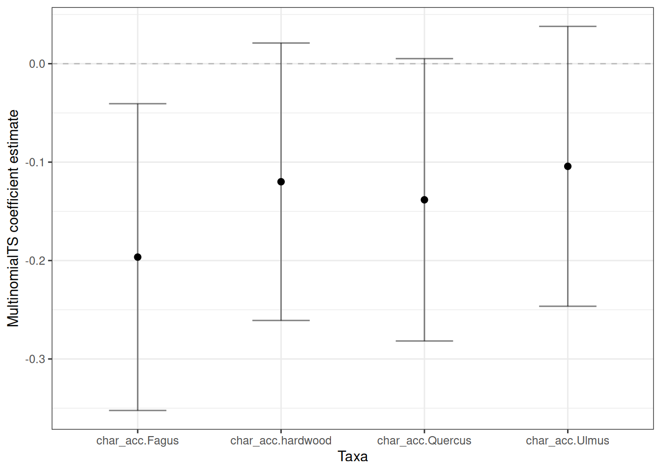

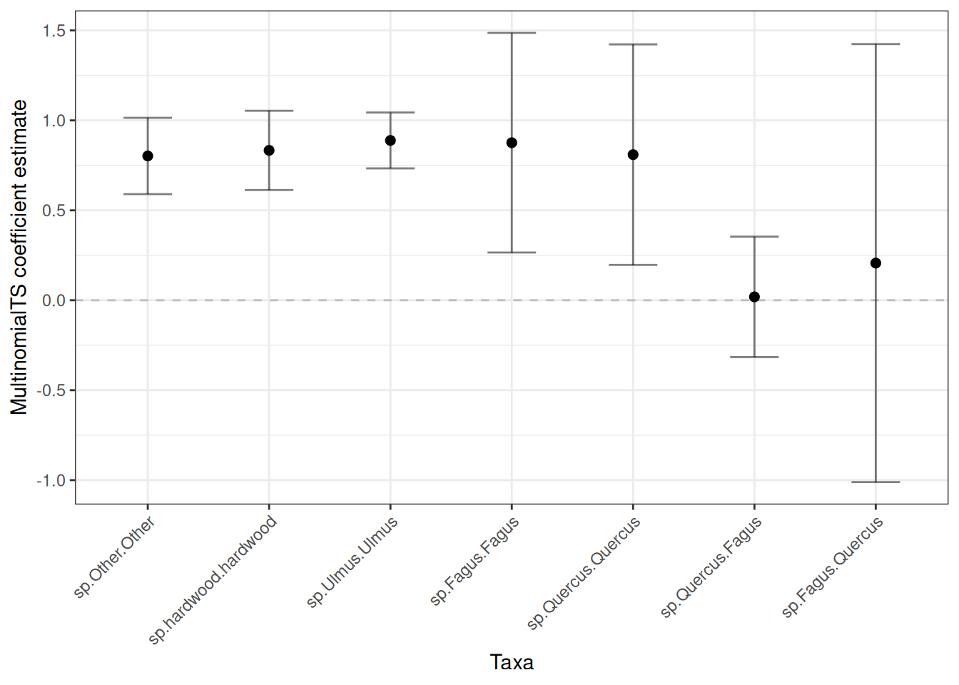
Now let’s grab the species coefficients:

plot_spp <- plot_boot |> 
  dplyr::filter(grepl("sp.*", name)) |>  mutate(name = factor(name,
    levels = c(
      "sp.Other.Other",
      "sp.hardwood.hardwood",
      "sp.Ulmus.Ulmus",
      "sp.Fagus.Fagus",
      "sp.Quercus.Quercus",
      "sp.Quercus.Fagus",
      "sp.Fagus.Quercus"
    )
  ))

ggplot(plot_spp, aes(x = name, y = boot_mean)) +
  geom_point(size = 2) +
  geom_hline(yintercept = 0, linetype = "dashed", alpha = 0.2) +
  geom_errorbar(aes(ymin = lower68, ymax = upper68),
                    width = .4, alpha = 0.5) +
  labs(x = "Taxa", y = "MultinomialTS coefficient estimate") +
  theme_bw() +
  theme(
        axis.text.x = element_text(angle = 45, hjust = 1)
  )

Since this is not a ggplot tutorial, we won’t go through stylising the plots. You probably have your own preferred design anyway! I have done this in dplyr and ggplot2, as they are currently very commonly used. However, other options such as data.table or plotly, or straight-up base R can also be used!

Introduction

This vignette

Data processing

State variables YY

Handling the covariates XX

Fitting multinomialTS

Finding initial conditions using mnGLMM()

Setting-up parameters for mnGLMM()

Fitting mnGLMM()

Setting-up parameters for mnTS()

Fitting mnTS()